t-Test
Published:
This post covers t-Tests.

t-Distribution
- Z - test works when we know $\mu$ and $\sigma$
- Use Samples
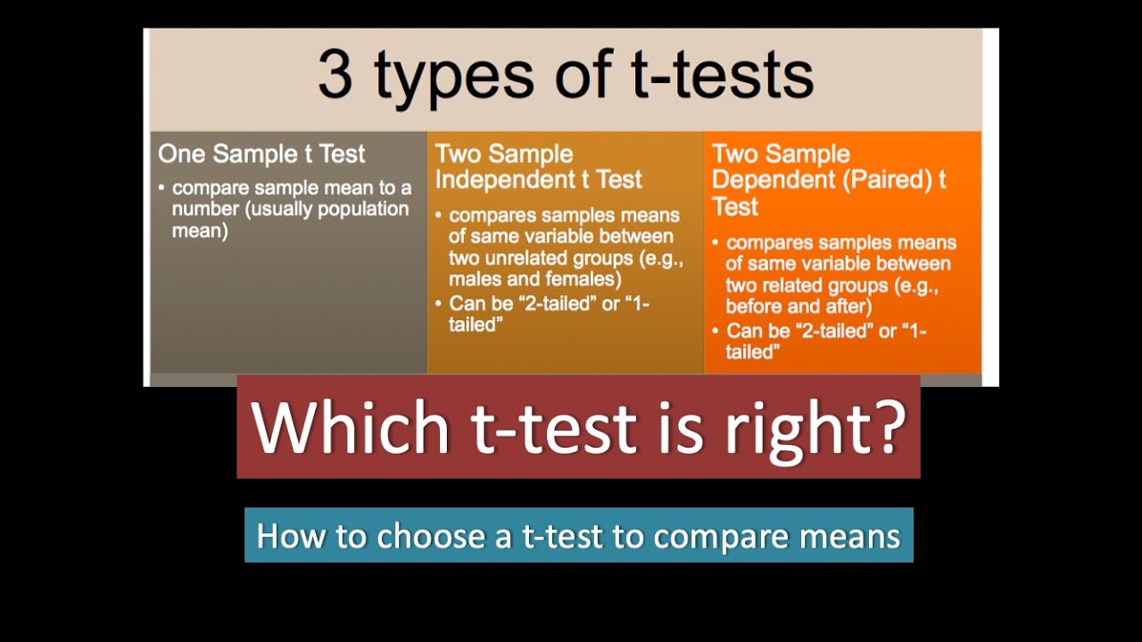
- How different a sample mean is from a population
- How different two sample means are from each other
- Two samples can be
- Independent
- Dependent
- Two samples can be
- Estimate Population Standard Deviation using sample standard deviation with Bessel’s correction
- Bessel’s correction is the use of $n − 1$ instead of $n$ in the formula for the sample variance and sample standard deviation, where $n$ is the number of observations in a sample.
- This method corrects the bias in the estimation of the population variance.
- It also partially corrects the bias in the estimation of the population standard deviation.
- However, the correction often increases the mean squared error in these estimations.
- This technique is named after Friedrich Bessel.
- To find out how typical or atypical (unusual) a sample mean - find its location on the distribution of sample means i.e. sampling distribution
- we can determine when we know population parameters, $\mu, \sigma$
- $ std~errro= \frac{\sigma}{\sqrt{n}}$
- $z = \frac{sample~mean - \mu}{std~error} = \frac{mean~difference}{std~error}$
- Std for Samples = $S = \sqrt{\frac{\Sigma(X_i - \bar{X})^2}{n-1}}$
- Standard Error depends on sample, we cannot use $\sigma$ if we have sample
- Thus, we have a new distribution that is more prone to error - t-Distribution
- more spread out and thicker in the tails than a normal distribution
- Since large sample sizes gives skinnier sampling distribution
- more spread out and thicker in the tails than a normal distribution
- What happens as n increases?
- The t-Distribution approaches to Normal Distribution
- The t-Distribution gets Skinnier tails
- $S \rightarrow \sigma$
Degree of Freedom - Sample Standard Deviation
- We can pick a sample of size $n$ from population using $n$ degrees of freedom
- Now to compute Standard Deviation, we need sample mean
- $\bar{X} = \frac{X_1+X_2+X_3+…+X_n}{n}$
- $ X_1+X_2+X_3+…+X_n = n . \bar{X} $
- $n-1$ Degrees of Freedom
- We may vary $n-1$ values to keep the sum of these values as $n\bar{X}$
- $n-1$ is the effective sample size since only $n-1$ values are independent if we know the mean.
- $S = \sqrt{\frac{\Sigma(X_i - \bar{X})^2}{n-1}}$
- As degrees of freedom increases, the t-distribution better approxiamate the normal distribution
t-Table
- https://naneja.github.io/python/t-table
- Questions
What’s the t-critical value for a one-tailed alpha level of 0.05 with 12 degrees of freedom.
- df = 11 and p = 0.05
- Ans t = 1.782
- df = 11 and p = 0.05
What are t-critical values for 2-tailed test with $\alpha = 0.05$ and sample size 30
- $df = 29,~ p = \pm 0.025$
- Ans: $\pm 2.045$
What are the limits for the right area of t-statistic when the sample size is 24 and the t-statistic is 2.45
- $df=23, t=2.45$
- $p = .02 ~\text{or}~ .01$
t-Statistic
$t = \frac{\bar{X}-\mu_0}{\frac{S}{\sqrt{n}}}$
- The larger/smaller the value of $\bar{X}$, the stronger the evidence that $\mu > \mu_0$
- The larger/smaller the value of $\bar{X}$, the stronger the evidence that $\mu < \mu_0$
- The further the value of $\bar{X}$ from $\mu_0$ in either direction, the stronger/weaker the evidence that $\mu \ne \mu_0$
|  |
|  | | ———————————————————— | ————————————- |
One Sample t-Test
$t = \frac{\bar{X}-\mu_0}{\frac{S}{\sqrt{n}}}$
\[H_0: \mu = \mu_0 \\\begin{align*} H_A &: \mu < \mu_0 \\ &: \mu > \mu_0 \\ &: \mu \ne \mu_0 \end{align*}\]$\alpha$ Levels (column levels of t-table)
- What will increase the t-Statistic
- Large difference between $\bar{X}$ and $\mu_0$
- Larger $n$
- Larger $S$
- Large Standard Error
- Larger t-Statistic
- => Lower probability of obtaining t-Statistic
- => Larger $\bar{X} - \mu_0$
P-Value
Compute t-statistic
- $t = \frac{\bar{X}-\mu_0}{\frac{S}{\sqrt{n}}}$
One-tailed Test
- p-value is the probability
- above the t-Statistic if it’s positive, or
- below the t-Statistic if it’s negative
- p-value is the probability
Two-tailed Test
- p-value is the probability of the sum of both
- above the t-Statistic and
- below the t-Statistic
- p-value is the probability of the sum of both
Reject the Null when the p-value is less than the $\alpha$ level
Example - Finches Beek Width
- Average known Beak Width = 6.07 mm
- $H_0: \mu = 6.07$
- $H_A: \mu \ne 6.07$
- Sample Size = 500
- Degrees of Freedom = 499
- Compute the sample mean and std dev from the sample dataset
- $\bar{X} = 6.470$
- $S = \sqrt{\frac{\Sigma(X_i - \bar{X})^2}{n-1}} = 0.396$
- t-Statistic
- $ t = \frac{6.47 - 6.07}{0.396/\sqrt{500}} = \frac{0.4}{0.0179} = 22.346$
- Table
- $df = 499,~ t = 22.346$, https://naneja.github.io/python/t-table
- $p = 0$
- Reject null
- probability of getting this t-value is very very small
- probability of getting the sample with beek width 6.47 from the population with mean 6.07 is very very small
Example
- Sample = [5, 19, 11, 23, 12, 7, 3, 21]
Is this sample mean significantly different from 10 at an alpha level of 0.05?
- Different => two-tailed t-test
- $n=8,~ \bar{X} = 12.625, S = 7.6$
- $t = \frac{\bar{X} - 10}{\frac{S}{\sqrt{n}}} = \frac{12.625 - 10}{\frac{7.6}{\sqrt{8}}} = 0.977$
- $df=7, t=0.977$
- https://naneja.github.io/python/t-table
- Two Tail Test
- $ p = 0.18 + 0.18 = 0.36 > 0.05 $
- Fail to Reject
- Thus, $H_0: \mu = 10$
Example
Mean Rent = 1830 for all apartments
Company A wants to know if the rent they are charging is significantly different at $\alpha = 0.05$
- Sample:
- $n=25,~ \bar{X}=1700,~ S=200$
- Sample:
Hypothesis
- $H_0: \mu = 1830$ and
- $H_A: \mu \ne 1830$
- What are t-critical values
- $t = \frac{\bar{X} - 1830}{\frac{S}{\sqrt{n}}} = \frac{1700 - 1830}{\frac{200}{\sqrt{25}}} = -3.250$
- $df = 24, t = -3.25 $
- Two Tail Test
- https://naneja.github.io/python/t-table
- $p = 0.0025 + 0.0025 = 0.005 < 0.05$
- Reject the null in favor of $H_A: \mu \ne 1830$
What is the Confidence Interval for the population for Company A?
95% Confidence Interval
For 95% CI, we need t-critical value at p=0.025 at df = 24
- $df=24, ~p=0.025 \implies t_{critical} = 2.064 $
- $\pm ~\text{t_critical} * \text{std_error} = t * \frac{S}{\sqrt{n}} $
- $2.064 * \frac{200}{\sqrt{25}} = 82.56$
- CI = $(1700 - 82.56, 1700 + 82.56) ~=~ (1617.44, 1782.56) $
Margin of Error = 82.56
If n = 100
What are t-critical values
- $t = \frac{\bar{X} - 1830}{\frac{S}{\sqrt{n}}} = \frac{1700 - 1830}{\frac{200}{\sqrt{100}}} = -6.50$
- $df = 24, t = 6.5 $
- https://naneja.github.io/python/t-table
- $p = 0.00 + 0.00 = 0.00 < 0.05$
Reject the null in favor of $H_A: \mu \ne 1830$
What is the Confidence Interval for the population for Company A? - 95% Confidence Interval
- $df = 99, p = 0.025 \implies t_{critical} = $ 1.984
- Margin of Error = $\pm ~\text{t_critical} * \text{std_error} = t_{critical} * \frac{S}{\sqrt{n}} $
- ME = $1.984 * \frac{200}{\sqrt{100}} = 39.68$
- Increase of sample size will reduce Margin of error
- CI = $(1700 - 39.68, 1700 + 39.68) ~=~ (1660.32, 1739.68) $
Cohen’s d
- Standardized mean difference that measures the distance between means in standardized units
- $Cohen’s~d = \frac{\bar{X}-\mu}{S}$
- In above Rent Example
- $\mu = 1830$
- Sample: $n = 25, \bar{X} = 1700, S = 200$
- $d = \frac{\bar{X}-\mu}{S} = \frac{1700 - 1830}{200} = -0.65$
Dependent Samples
Same subject takes the test twice
Within subject designs
- each subject is assigned two conditions in random order
in control but get treatment
two kinds of treatment
Every subject is given a Pre-Test and a Post-Test
- Growth over time (Longitudinal Study)
- Each subject at different points of time
xi yi Di = xi - yi x1 y1 D1 = x1-y1 x2 y2 D2 = x2-y2 x3 y3 D3 = x3-y3 - each subject is assigned two conditions in random order
Example - Keyboards
- Errors in two design of keyboards (QWERTY and Alphabetical)
- https://naneja.github.io/datasets
- file = Keyboards.csv
- https://naneja.github.io/datasets
- Mean Error
- n = 25
- Querty Keyboard = 5.08 and
- Alphabetical Keyboard = 7.8
Are these differences significant?
- $n = 25$
$H_0: \mu_Q = \mu_A ~and~ H_A: \mu_Q \ne \mu_A$
- Also can say $\mu_Q - \mu_A = 0$
What is Point Estimate for $\mu_Q - \mu_A$
- $\mu_Q - \mu_A = 5.08 - 7.8 = -2.72$
What is S
- d = QWERTYerrors - Alphabeticalerrors
- std_dev = $S = s_d = \sqrt{\frac{\Sigma (d-\bar{d})^2}{N-1}}$
- 3.69
- What is t-Statistic when S = 3.69
- $t = \frac{\mu_Q - \mu_A}{\frac{S}{\sqrt{n}}} = \frac{5.08 - 7.8}{\frac{3.69}{\sqrt{25}}} = -3.69$
- What is p-value
- Two Tail Test
- $df=24, t = -3.69$
- https://naneja.github.io/python/t-table
- $ p = 0.0005 + 0.0005 = 0.001 < 0.05 $
- Two Tail Test
Reject the Null or Fail to reject Null
- Reject the Null
- Significant Less Error and we may say causal effect due to keyboard design
- 95% Confidence Interval
- What are t-Critical Values for $\alpha=0.05$
- $ df = 24, p = 0.025$
- $t_{critical} = \pm 2.064$
- point estimate$ = \mu_Q - \mu_A = 5.08 - 7.8 = -2.72$
- $CI = \text{point estimate} \pm t_{critical} * \text{std error}$
- $CI = -2.72 - 2.064 * \frac{3.69}{\sqrt{25}}, ~ -2.72 + 2.064 * \frac{3.69}{\sqrt{25}}$
- -4.24, -1.20
- Users will make fewer errors in the range of 4 to 1 on querty keyboard than alpha errors
- What are t-Critical Values for $\alpha=0.05$
Advantages and Disadvantages- Dependent Samples
- Within-Subject design
- Two Conditions
- Longitudinal
- Pre-Test, Post-Test
- Advantages
- Controls for individual differences
- Use Fewer Subjects
- Cost-Effective
- Less Time-consuming
- Less Expensive
- Disadvantages
- Carry-over Effects
- Second measurement can be affected by first treatment
- Order may influence results
- Within-Subject design
Independent Samples
- Between-Subject Designs
Experimental
Observational
$ t = \frac{\bar{X_1}-\bar{X_2}}{standard~error} $
Standard Deviation = $\sqrt{S_1^2 + S_2^2}$
- We can’t take differences since these are not the same subjects (independent samples)
Standard Error $ = \frac{S}{\sqrt{n}} = \frac{\sqrt{S_1^2 + S_2^2}}{\sqrt{n}} = \sqrt{\frac{S_1^2 + S_2^2}{n}} = \sqrt{\frac{S1^2}{n} + \frac{S2^2}{n}} = \sqrt{\frac{S1^2}{n_1} + \frac{S2^2}{n_2}}$
Degrees of Freedom $ df= (n_1-1) + (n_2-1) = n_1 + n_2 -2$
- $ t = \frac{(\bar{X_1}-\bar{X_2})}{SE}$
Example - Food Prices
- https://naneja.github.io/datasets
- file = FoodPrices.csv
- Hypothesis
- $H_0 : \mu_1 = \mu_2$
- $H_A : \mu_1 \ne \mu_2$
- $n1 = 18,~ n2 = 14$
- $df = n1 + n2 - 2 = 30$
- Sample Mean and Std Dev
- $\bar{X_1} = 8.94,~ \bar{X_2} = 11.14$
- $S_1 = 2.65,~ S_2 = 2.18$
- $S = \sqrt{\frac{S1^2}{n_1} + \frac{S2^2}{n_2}} = \sqrt{\frac{2.65^2}{18} + \frac{2.18^2}{14}} =0.85$
- $t = \frac{\bar{X_1} - \bar{X_2}}{S} = \frac{8.94 - 11.14}{0.85} =2.58$ (Ignore negative sign)
- $df = 30,~ t = 2.58$
- $p = 0.01 + 0.01 = 0.02 < 0.05$
- Reject the Null
- Prices are significantly different for both areas
|  | | ——————————————————— |