This post covers introduction to Image Classification using Deep Learning.

Image Classification

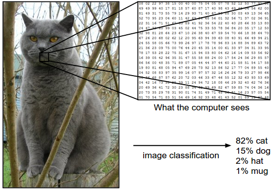Source: https://cs231n.github.io/assets/classify.png

• Total Numbers are $ w * h * c$

• Image Classification is $ f(w * h * c) = label $ or probability distribution $ f(w * h * c) = p_{l1}, p_{l2}, p_{l3}, ..p_{lK} $

• Challenges: Viewpoint Variation; Scale Variation; Deformation; Occlusion; Illumination conditions; Background clutter, Intra-class Variation

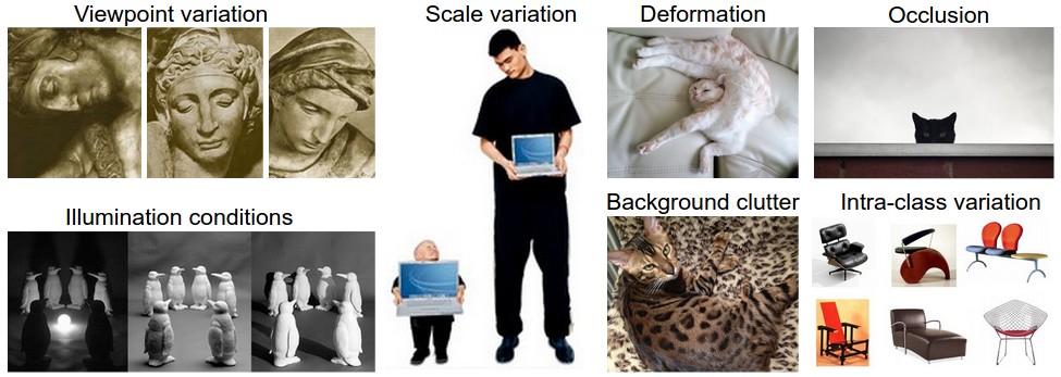
  • Source: https://cs231n.github.io/assets/challenges.jpeg

• Solution: Data-driven Approach

• Pipeline

  • Input: Training Set with $ N $ images, each labeled with one of $ K $ different classes.
  • Learning: Training a model/classifier
  • Evaluation: predict labels for images that have not been used for training

Nearest Neighbor Classifier

• CIFAR-10
  • Training Set: $50,000 * 32 * 32 * 3 $
  • Test Set: $10,000 * 32 * 32 * 3 $
  • Classes: 10 (5000 images of each class)

• L1 distance

  • $ d_1(I_1, I_2) = \sum\limits_{pixels}abs(I_1^p - I_2^p) $

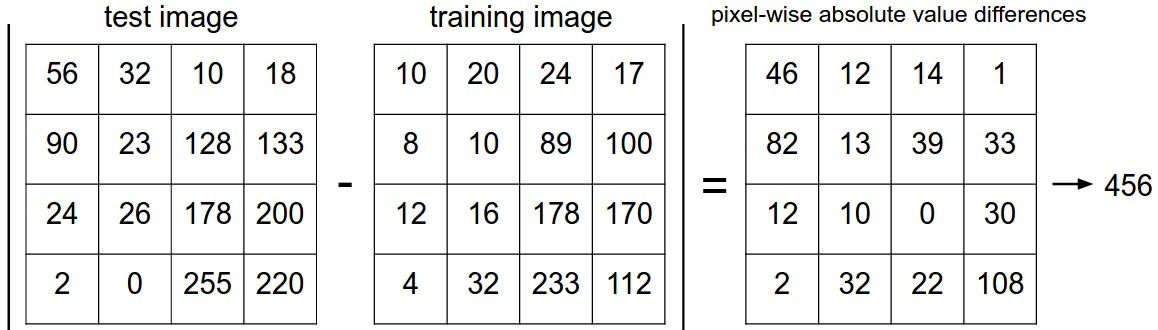
• Source: https://cs231n.github.io/assets/nneg.jpeg

• L2 distance

  • $ d_2(I_1, I_2) = \sqrt( \sum\limits_{pixels}(I_1^p - I_2^p) ^2 ) $

X_train, y_train, X_test, y_test = load_CIFAR10(path)
X_train  = X_train.reshape(50000, 32*32*3)
X_test  = X_test.reshape(10000, 32*32*3)
nn = NearestNeighbor()
nn.train(X_train, y_train)
y_test_predict = nn.predict(X_test)
accuracy = np.mean(y_test_predict == y_test)

• k - Nearest Neighbor Classifier
  • Instead of finding single closest images in the training set, we can find top $ k $ closest images and have them vote on the label of the test image. Higher values of $ k $ will give better results and makes the classifier resistant to outliers.
• Validation sets for Hyperparameter tuning
  • Choosing $L_1$ or $L_2$ distance
  • Choosing the value of $k$ for k-Nearest Neighbor
  • Test set must not be used for tweaking hyperparameters rather use validation set by splitting training set
  • Observe the accuracy of valid dataset for different values of k
  • Test Dataset to be used at the end and to report performance
• Cross-validation
  • k-folds cross validation
    • split the dataset in $k$ equal folds
    • Use $k-1$ for training and $1$ for validation
    • iterate the sets and average the performance
    • provides less noisy and better estimates but time Consuming so ok if the dataset is small
• Analysis Nearest Neighbor classifier
  • No Train Time
  • High Computation Cost at testing
  • Good choice if data is low dimensional but is rarely useful in image classification

Linear Classification

• Score Function: maps raw data to class scores, $ f(w * h * c) = p_{l1}, p_{l2}, p_{l3}, ..p_{lK} $

• Loss Function: quantify agreement between predicted scores and ground truth labels

• Parameterized mapping from images to label scores
  • Training dataset of images $x_i \in R^D,~ where ~i=1…N$ each associated with a label $y_i$, where $y_i \in 1…K$
  • $N$ examples with $D$ dimensionality and $K$ distinct categories
  • Score Function $f : R^D -> R^K$, maps raw pixels to class scores
• Linear Classifier

  • $ f(x_i, W, b) = Wx_i + b $, where $ x_i $ flattened to $ X_{D * 1} $ and $ W_{K * D} $ and $ b_{K * 1} $

  • $ W_{K * D} * X_{D * 1} + b_{K * 1} -> y_{K * 1}$

  • Parameters in W are called Weights and $b$ is bias vector since $b$ influences score without interlacing with actual data

  • $ W $ has $ K $ rows and is effectively evaluating $ K $ classifiers in parallel (one for each class) i.e. each classifier is a row of $W$

  • Linear classifier computes the score as a weighted sum of all pixels

  • $K$ classifiers implies $K$ straight lines that classifies $ K $ categories, can be visualized if $D$ dimensions be squashed in 2 dimensions.

  • $W$ is template or prototype

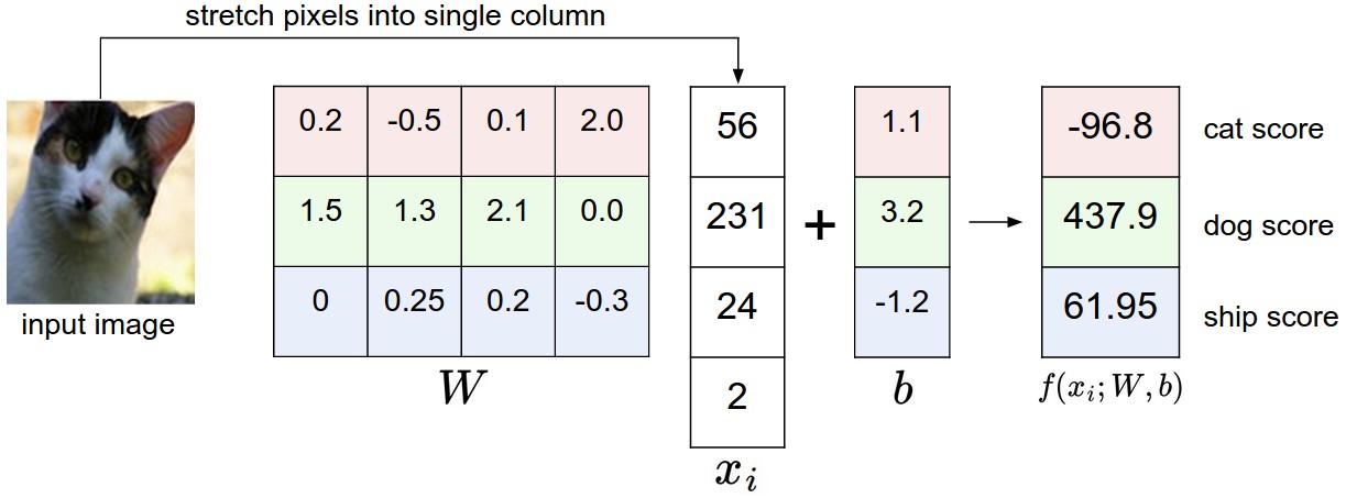
    Source: https://cs231n.github.io/assets/imagemap.jpg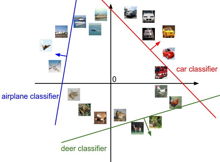

  • Source: https://cs231n.github.io/assets/pixelspace.jpeg

• Bias Trick

  • $f(X, W) = W*X$ -> combine W and b and add constant $1$ dimension to $X$

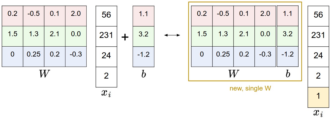
    Source: https://cs231n.github.io/assets/wb.jpeg

• Image Data Processing
  • Perform Normalization of Features to center the data by subtracting mean from every feature
    • Mean image is computed across the training images [0, 255] - 127 -> [-127, 128]
  • Scale each input feature so that values range from [-1, 1]
  • Zero mean centering is important for Gradient Descent
• Multiclass Support Vector Machine (SVM) Loss
  • SVM wants correct class score for each image must be higher than incorrect correct class by fixed margin $ \varDelta $
  • Let $ s = f(x_i, W) = W*x_i$ be the score function, thus $ s $ is a vector of $ K $ dimensions and each element of $ s $ represents score of each class

• Score of $j-th$ class is the $ j-th $ element, $ s_j = f(x_i, W)_j $

• One of the element of $ s_j $ is correct class, say $ s_{y_i} $, this we want to have higher value than all other incorrect classes. If it is already higher than margin then we want to have loss as zero for zero contribution from that particular class

• Thus, if $ s_j + \varDelta - s_{yi} < 0 $ -> zero contribution to loss

• if $ s_j + \varDelta - s_{yi} > 0 $ -> positive contribution to loss

• $ L_i = \sum\limits_{ j \neq y_i } max(0, s_j + \varDelta - s_{y_i} ) $

• Example:
  • $ s = [13, -7, 11] $ and first class is the true class i.e $ y_i = 0 $ and let $ \varDelta = 10 $
  • Although 13 is greater than -7 and 11 but need to check if it is greater than margin
  • $ L_i = max(0, -7 + 10 - 13) + max(0, 11 + 10 - 13) = 0 + 8 = 8 $
• In case of Linear Classifiers, the loss function can be written as:
  • $ L_i = \sum\limits_{ j \neq y_i } max(0, w_j^T * x_i + \varDelta - w_{ y_i }^T * x_i ) $
  • $ w_j $ is the $ j-th $ row of W reshaped as column

Hinge Loss

• Loss function threshold at zero i.e. $ max (0, _) $ is called hinge loss
• Squared hinge loss is $ max (0, - ) ^ 2 $, also called L2 - SVM, penalises violated margins more strongly

Regularization

• Let we learned $ W $ for which $ L_i = 0~\forall~i $. The issue is that this $ W $ is not unique e.g. if $ W $ gives zero loss then $ \lambda * W $ will also give zero score for $ \lambda > 1$ since the transformation uniformly stretches all score magnitudes and hence their absolute differences.
  • If difference between correct class and incorrect class is $2$ then multiplying $W$ by 2 will make that difference $4$
• To remove this ambiguity, we want to encode some preference for a certain set of weights over others
• We extend the loss function with regularization penalty $ R(W) $ e.g. L2 norm that discourages large weights
  • $ R(W) = \sum\limits_{k} \sum\limits_{l} W_{k,l}^2$
  • Regularization function is not dependent on the data
• Multiclass Support Vector Machine (SVM) Loss now have two components
  • Data Loss i.e. Average loss for all examples $ \frac{\sum L_i}{N} $
  • Regularization Loss, $ R(W) $
• $ L = \frac{\sum L_i}{N} + \lambda * R(W) $, where $ \lambda $ is weighted parameter to be determined from cross validation
• $ L = \frac{1}{N}*{\sum\limits_{ j \neq y_i } max(0, w_j^T * x_i + \varDelta - w_{ y_i }^T * x_i )} + \lambda * \sum\limits_{k} \sum\limits_{l} W_{k,l}^2 $

Example

• L2 Regularization improves generalization by penalizing large weights so that no input dimensions can have large influence
• x = [1, 1, 1, 1]
• $ w_1 = [1, 0, 0, 0] $ and $ w_2 = [0.25, 0.25, 0.25, 0.25] $ are two weight vectors for one class
• Now, $ W_1^T * x = W_1^T * x = 1 $, same score
• L2 Penalty for $w_1$ is $1^2 + 0^2 + 0^2 + 0^2 = 1$ and for $w_2$ is $0.25^2 + 0.25^2 + 0.25^2 + 0.25^2 = 0.25 $
• Thus, $w_2$ has lower L2 penalty so better weight due to better diffusion.
• Results less overfitting

Bias

• As biases don’t control influence of an input dimension, we only need to regularize weights $W$ and not $b$, however it has negligible effect
• Due to regularization, we will not get zero loss, since $R(W)$ can only be zero when when all weights are zero

Practical Considerations

• Setting Delta and Lambda
  • $ \Delta $ can be safely set to $ 1.0 $
  • Both hyperparameters $ \Delta $ and $ \lambda $ control the same tradeoff
  • Magnitude of $W$ will effect scores and score differences and lower values of $W$ will result in low score differences.
  • Thus, exact value of $ \Delta = 1 ~or~ \Delta = 100 $ is meaningless since weights can shrink or stretch the differences
  • Real tradeoff is how large we allow the weights to grow (via $\lambda$ )
• Relation to Binary SVM
  • For intended output $ t = \pm 1 $ and classifier score $y$, the hinge loss of pred $y$ is $ L = max(0, 1 - t * y ) $. Now t is the truth value that can be -1 or +1 and y is the predicted value e.g. in linear SVM, $ y=w * x + b $.
  • If $ y $ and $ t $ both have same sign, means prediction is correct ($ 1-ty < 0 $) and when these have opposite signs then prediction is incorrect ($ 1-ty > 0 $)
  • Even if both have same sign but when $ abs(y) < 1$ then also $1-ty > 0$, so will try to increase margin
  • We use, $ L_i = C * max(0, 1 - y_i * w^T * x_i) + R(W) $, $C$ is a hyperparameter and where $ C \alpha \frac{1}{\lambda} $, where $y_i \pm 1$
• Other Multiclass SVM
  • One-Vs-All (OVA) SVM trains independent binary SVM for each class vs all other classes, In Defense of One-Vs-All Classification
  • Structured SVM, maximizes the margin between score of correct class and score of the highest-scoring incorrect runner-up class

Softmax Classifier

• Softmax is generalization form of Binary Logistic Regression Classifier for multiple classes

• While SVM treats output of $ f(x, W) $ as scores, Softmax provides normalized probabilities by interpreting output as unnormalized log probabilities and replace hinge loss with cross-entropy loss:

• Cross Entropy Loss = $ L_i = -log \left(\frac{ e^{f_{y_i} }}{ \sum\limits_{j} e^{f_j} }\right) $

• Cross Entropy Loss = $ L_i = -f_{y_i} + log \sum\limits_{j} e^{f_j} $

• This is softmax function and full loss is average loss for all examples and regularization penalty

• Information Theory View

  • Cross-entropy between true distribution $ p $ and estimated distribution $ q $:
    • $ H(p,q) = - \sum\limits_{x} p(x) \log q(x) $
    • $ p = [ 0, …1, …,0 ] $ and $ q = e^{f_{y_i}} / \sum\limits_{j} e^{f_j} $

• Probabilistic Interpretation

  • $ P(y_i \mid x_i; W) = \frac{e^{f_{y_i}}}{\sum\limits_{j} e^{f_j} } $ - is normalized probability for $y_i$ give $ x_i $ and parameterized by $ W $
  • Since, we interpret model output as unnormalized log probabilities, thus we are minimizing the negative log likelihood of the correct class - Maximum Likelihood Estimation (MLE).

• Numerical stability

  • Softmax $ \frac{e^{f_{y_i}}}{\sum\limits{j} e^{f_j}} $ can be numerically unstable when the values are large, thus we may rewrite it as:
    • $ \frac{Ce^{f_{y_i}}}{C\sum e^{f_j}} = \frac{e^{f_{y_i} + \log C}}{\sum e^{f_j + \log C}} $
    • $ C $ can be any value, we choose $ C $ so that it is negative maximum value to make highest value zero
    • Thus, we shift the values to left so that maximum is zero and then compute softmax
  • Naming Conventions
    • SVM Classifier uses Hinge Loss or also called max-margin loss
    • Softmax Classifier uses Cross Entropy Loss
  • SVM vs Softmax Example
    • Let $W*x_i = [ -2.85, 0.86, 0.28] $, where correct class $ y_i = 2 $
    • Hinge Loss (SVM): $ max(0, -2.85+1-0.28) + max(0, 0.86+1-0.28) = 1.58 $
    • Cross Entropy Loss (Softmax)
      • Use exp function $ [e^{-2.85}, e^{0.86}, e^{0.28} ] = [0.058, 2.36, 1.32] $
      • Normalize $ [0.016, 0.631, 0.353] = 1.04 $
    • Loss numbers are not comparable and only meaningful within the same classifier
  • Probabilities in Softmax Classifier
    • How peaky or diffused these probabilities are depend on the regularization strength $ \lambda $
    • $ [1, -2, 0] -> [e^1, e^{-2}, e^0] = [2.71, 0.14, 1] -> [0.7, 0.04, 0.26] $
    • $ [0.5, -1, 0] -> [e^{0.5}, e^{-1}, e^0] = [1.65, 0.37, 1] -> [0.55, 0.12, 0.33] $
    • When $ \lambda $ is higher the weights will be penalized to have higher values and this will lead to lower values say half of previous -> probailities will change
    • Probabilitiies are more diffused in [0.55, 0.12, 0.33] than [0.7, 0.04, 0.26], and further the probabilities will be tiny and will be near uniform. Thus, these are confidence scores where order matters as in SVM rather than absolute numbers or differences.
  • SVM and Softmax are comparable
    • SVM has a local objective that may be feature or bug, once satisfied than correct class is higher than incorrect by margin, it will give zero loss
    • Scores [10, -2, 3] with first correct class and margin 1 will compute zero loss
    • Scores [10, -100, -100] or [10, 9, 9] will also give zero loss
    • Softmax is never fully happy [10, 9, 9] will give higher loss than [10, -100, -100]
    • However, this can be thought of as feature e.g. car classifier that is spending efforts on separating cars from trucks should not be influenced by frog, which it already assigned low scores