Chapter 2: Statistical Learning

Chapter 3: Linear Regression

Chapter 4: Logistic Regression

the response variable is qualitative

An Overview of Classification

• In the Defaults dataset, 3% of users default, and we can predict if the user will default based on balance and income.

Why not Linear Regression

• We can encode the values to numeric. However, the difference between numerals will not correspond to the difference between values. In some cases, it may be true, but not in general.

• For binary, we can use a dummy variable $0/1$ and can fit a linear regression and predict $val1 ~if~ \hat{Y} > 0.5$

  • However, linear regression values can be more than one, so it is hard to interpret.

  ## Logistic Function:

• Dataset: Defaults

  • Response Variable: default

  • Probability of default given balance = $Pr(default = Yes

    balance)$ or $p(balance)$ will range between $0$ and $1$.

  • If $p(balance) > 0.5$ then default, or the company may also choose $p(balance) > 0.1$ as default

Logistic Model

• How to model $p(X) = Pr(Y = 1

  X)$​

  • We can use $0/1$ encoding for response and apply linear regression

  • \[p(X) = \beta_0 + \beta_1X\]

  • However, some values of response can be -ve or greater than $1$. Thus, we need a function that gives values between $0$ and $1$. In Logistic Regression, we use Logistic Function

  • Logistic Function:

  • • use $exponential$ to convert all -ve to +ve
  \[p(X) = \frac{e^{\beta_0 + \beta_1X}}{1 + e^{\beta_0 + \beta_1X}}\]

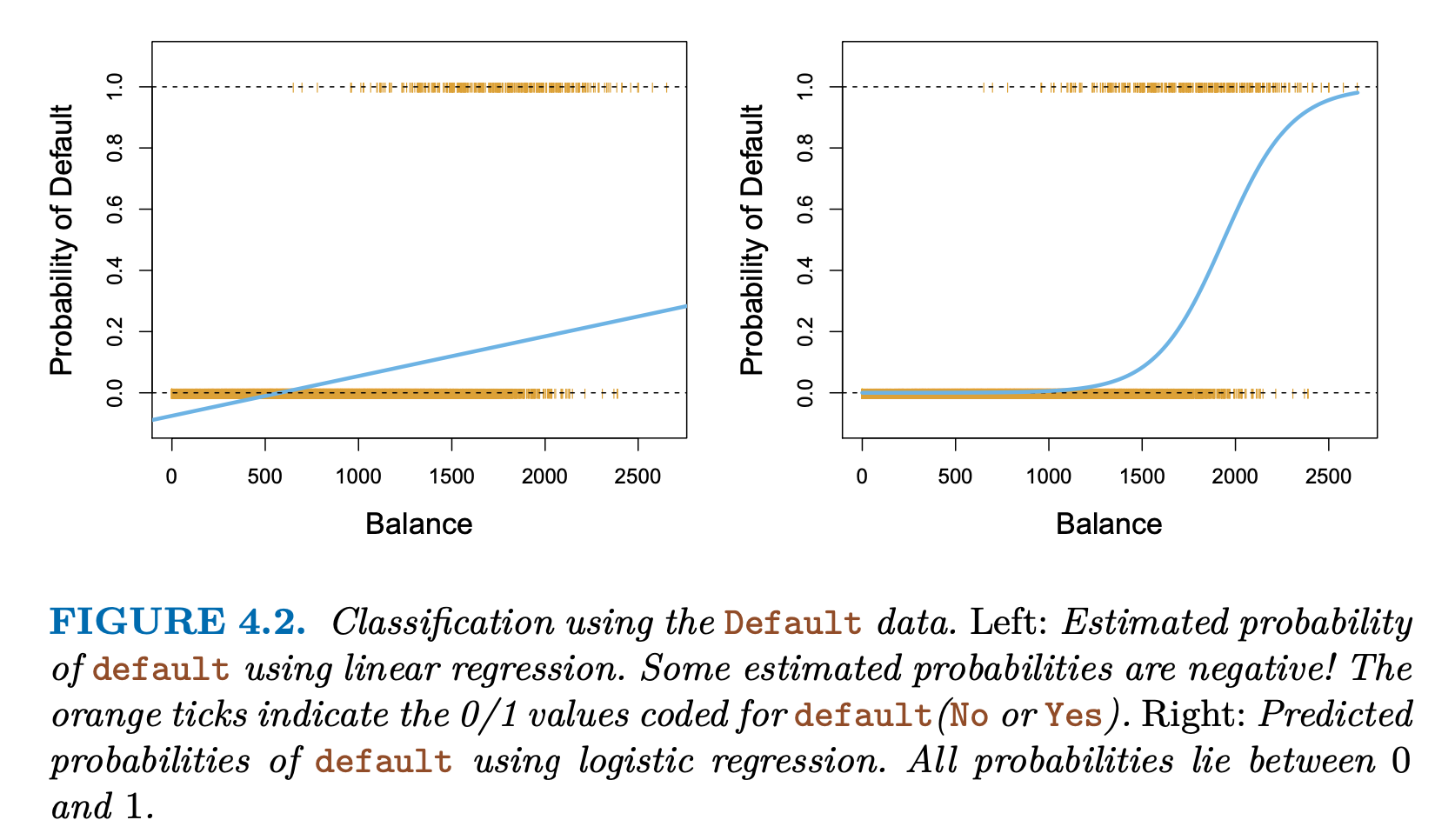
  left using linear regression with 0/1 and right using logistic regression (S curve)

  • For low balances, the prob is now close to $0$ and for high balance, it is close to $1$
  • Logistic Regression will always produce $S$ curve. Thus, sensible probs, regardless of the values of $X$

• We also find

  • \[\frac{p(X)}{1-p(X)} = e^{\beta_0 + \beta_1X}\]

  • The $\frac{p(X)}{1-p(X)}$ is called $odds$ and can take any values $0$ to $\infty$.

    • Odd $0$ means low prob and $\infty$ means high prob
    • On average 1 in 5 person will default.
      • $p = \frac{1}{5} = 0.2 \implies odds = \frac{0.2}{0.8} = \frac{1}{4}$
      • On average 1 in 5 persons will default with odds of 1/4
    • On average 9 in 10 person will default.
      • $p = \frac{9}{10} = 0.9 \implies odds = \frac{0.9}{0.1} = 9$
      • On average 9 in 10 persons will default with odds of 9
  • \[\text{Log Odds or Logits} = log\left[\frac{p(X)}{1-p(X)}\right] = \beta_0 + \beta_1X\]
    • Logit is linear in X
      • increasing $X$ by one unit
        • changes the log odds by $\beta_1$
        • or multiply the odds by $e^{\beta_1}$

Estimating the Regression Coefficients

• maximum likelihood is preferred for Logistic Regression

  • Estimate $\beta_0$ and $\beta_1$ such that the predicted probability $\hat{p}(x_i)$ of default matches with individuals

• $likelihood ~function$:

  • \[\mathcal{l} (\beta_0, \beta_1) = \prod_{y_i=1}p(x_i) \prod_{y_i'=0}[1-p(x_i')]\]
  • The estimates $\hat{\beta_0}$ and $\hat{\beta_1}$​ are selected to maximize the likelihood function.

y = df.default == "Yes" # y is a boolean

X = ["balance"]
X = MS(X).fit_transform(df)

model = sm.GLM(y, X, family=sm.families.Binomial()).fit()

display(summarize(model))

• a one-unit increase in balance is associated with an increase in the log odds of default by 0.0055 units.
• The z-statistic plays the same role as the t-statistic in the linear regression output.
• There is indeed an association between balance and the probability of default. The estimated intercept is typically not of interest; its main purpose is to adjust the average fitted probabilities to the proportion of ones in the data (in this case, the overall default rate).

Making Predictions

• What is the probability for an individual with a balance of $1000?

  • $X = 1000$
  • $\beta_0 = -10.6513$ and $\beta_1 = 0.0055$
  • $\hat{p}(X) = \frac{e^{\hat{\beta_0} + \hat{\beta_1}X}}{1 + e^{\hat{\beta_0} + \hat{\beta_1}X}} = 0.00576$
  • Less than 1%

• What is the probability for an individual with a balance of $2000?

  • $X = 2000$
  • $\beta_0 = -10.6513$ and $\beta_1 = 0.0055$
  • $\hat{p}(X) = \frac{e^{\hat{\beta_0} + \hat{\beta_1}X}}{1 + e^{\hat{\beta_0} + \hat{\beta_1}X}} = 0.586$
  • 58.6 %

•   import numpy as np
    X = 1000
    beta_0 = -10.6513
    beta_1 = 0.0055
    y = beta_0 + beta_1 * X
    p = np.exp(y) / (1 + np.exp(y))
    print(p)
  

y = df.default == "Yes" # y is a boolean

X = ["student"]

df["student"] = df["student"].astype('category')

X = MS(X).fit_transform(df)

model = sm.GLM(y, X, family=sm.families.Binomial()).fit()
display(summarize(model))

• If you are a student, log odds will increase by 0.40 and the p-value is high. This indicates that students tend to have higher default probabilities than non-students

• What is the probability of default if the Student

  • $Student[Yes] = 1$
  • $\beta_0 = -3.5041$ and $\beta_1 = 0.4049$
  • $\hat{p}(X) = \frac{e^{\hat{\beta_0} + \hat{\beta_1}X}}{1 + e^{\hat{\beta_0} + \hat{\beta_1}X}} = 0.04314$
  • 4%

• What is the probability of default if the not a Student

  • $Student[Yes] = 1$
  • $\beta_0 = -3.5041$ and $\beta_1 = 0.4049$
  • $\hat{p}(X) = \frac{e^{\hat{\beta_0} + \hat{\beta_1}X}}{1 + e^{\hat{\beta_0} + \hat{\beta_1}X}} = 0.02919$
  • 2.9%

•   import numpy as np
    studen_yes = 0
    beta_0 = -3.5041
    beta_1 = 0.4049
    y = beta_0 + beta_1 * studen_yes
    p = np.exp(y) / (1 + np.exp(y))
    print(p)
  

Multiple Logistic Regression

y = df.default == "Yes" # y is a boolean

X = ["balance", "income", "student"]

df["student"] = df["student"].astype('category')

X = MS(X).fit_transform(df)

model = sm.GLM(y, X, family=sm.families.Binomial()).fit()
display(summarize(model))

• Analysis

  • balance and student are associated with the default
    • students are less likely to default since coefficient is negative (surprising result)
      • The overall student default rate is higher than the non-student default rate
      • The negative coefficient for student in the multiple logistic regression indicates that for a fixed value of balance and income, a student is less likely to default than a non-student.
  • A student is riskier than a non-student if no information about the student’s credit card balance is available. However, that student is less risky than a non-student with the same credit card balance!

• Confounding

  • Results obtained using one predictor may differ from those obtained using multiple predictors, especially when there is a correlation among the predictors.

• Predictions

  •   intercept = model.params["intercept"]
            
      beta_balance = model.params["balance"]
      beta_income = model.params["income"]
      beta_student_yes = model.params["student[Yes]"]
            
      X_balance = 1500
      X_income = 40 # for 40K as per the table
      X_student_yes = 1
            
      y = intercept + beta_balance * X_balance + beta_income * X_income + beta_student_yes * X_student_yes
      p = np.exp(y) / (1 + np.exp(y))
      print(p)
    

  • A student with a credit card balance of $1,500 and an income of $40,000

    • intercept = -10.869000

    • beta_balance = 0.005700; beta_income = 0.000003; beta_student_yes = -0.646800

    • X_student_yes = 1; X_balance = 1500; X_income = 40

    • \[p(X) = \frac{e^{\beta_0 + \beta_1X_1 +...+ \beta_1X_1}}{1 + e^{\beta_0 + \beta_1X_1 +...+ \beta_1X_1}} = 0.052\]
    • 5.2%

  • A non-student with a credit card balance of $1,500 and an income of $40,000

    • $p(X) = 0.105$
    • 10.5%

Multinomial Logistic Regression

more than two classes in the response variable

home = os.path.join(os.path.expanduser("~"), "datasets", "ISLP")
df = pd.read_csv(os.path.join(home, "Default.csv"))

y = df.default # y is not a boolean

X = ["balance", "income", "student"]

df["student"] = df["student"].astype('category')

X = MS(X).fit_transform(df)

model = sm.MNLogit(y, X).fit()
display(summarize(model))
summarize(model).to_latex()