This post covers Optimization and Backpropogation from cs231n.

Introduction

Problem Statement

• Given a function $f(x)$ where $x$ is a vector of inputs, compute gradient of $f$ at $x$ i.e. $\Delta f(x)$.

Motivation

• In case of Neural Networks, $f(x)$ corresponds to loss function and inputs $x$ consist of training data, network weights and bias.
• As $x$ is fixed, we compute gradient for $W$ and $b$ to use it for parameter update
• Gradient on $x_i$ is useful for visualization and interpret neural network learning

Simple Expression and Interpretation of gradient

• Let $f(x,y) = xy$ then $\frac{\partial f}{\partial x}=y$ and $\frac{\partial f}{\partial y}=x$

  • Derivative indicate rate of change of a function wrt the variable surrounding an infinitesimally small region near a particular point.

  • Let $x=4,~y=-3$, then $f(x,y) = -12$ and $\frac{\partial f}{\partial x}=-3$

    • This tells us that if we increase $x$ by tiny amount, then the whole expression will reduce by three times the tiny amount

  • $\frac{\partial f}{\partial y}=4$

    • This tells us that if we increase $y$ by tiny amount, then the whole expression will increase by four times the tiny amount

  • The derivate on each variable tell us the sensitivity of the whole expression on its value

  • Thus, $\Delta f = [\frac{\partial f}{\partial x}, \frac{\partial f}{\partial y}] = [y, x]$

• Let $f(x,y) = x+y$ then $\frac{\partial f}{\partial x}=1$ and $\frac{\partial f}{\partial y}=1$

  • $\Delta f = [\frac{\partial f}{\partial x}, \frac{\partial f}{\partial y}] = [1, 1]$
  • Incresing either $x$ or $y$ at any point, will increase output of $f$, the rate of increase is independent of the values of $x$ and $y$

• Let $f(x,y) = max(x,y) = x ~or~ y$

  • $ x >= y \implies max(x,y) = x ~and~ \frac{\delta f}{\delta x} = 1,~ \frac{\delta f}{\delta y} = 0$
  • $ y >= x \implies max(x,y) = y ~and~ \frac{\delta f}{\delta x} = 0,~ \frac{\delta f}{\delta y} = 1$
  • Subgradient is $1$ on the input that was larger and $0$ otherwise.
  • If the inputs are $x=4, y=2$, then max is $4$ and function is not sensitive of $y$ i.e. if we increase $y$ i.e. $2$, the value of the function will still be $4$, unless $h$ is larger than 2.
  • The derivative doesn’t tell us about large changes and these are informative for tiny, infinitesimals small changes on the input $lim_{h\to 0}$

Compound Expressions with Chain Rule

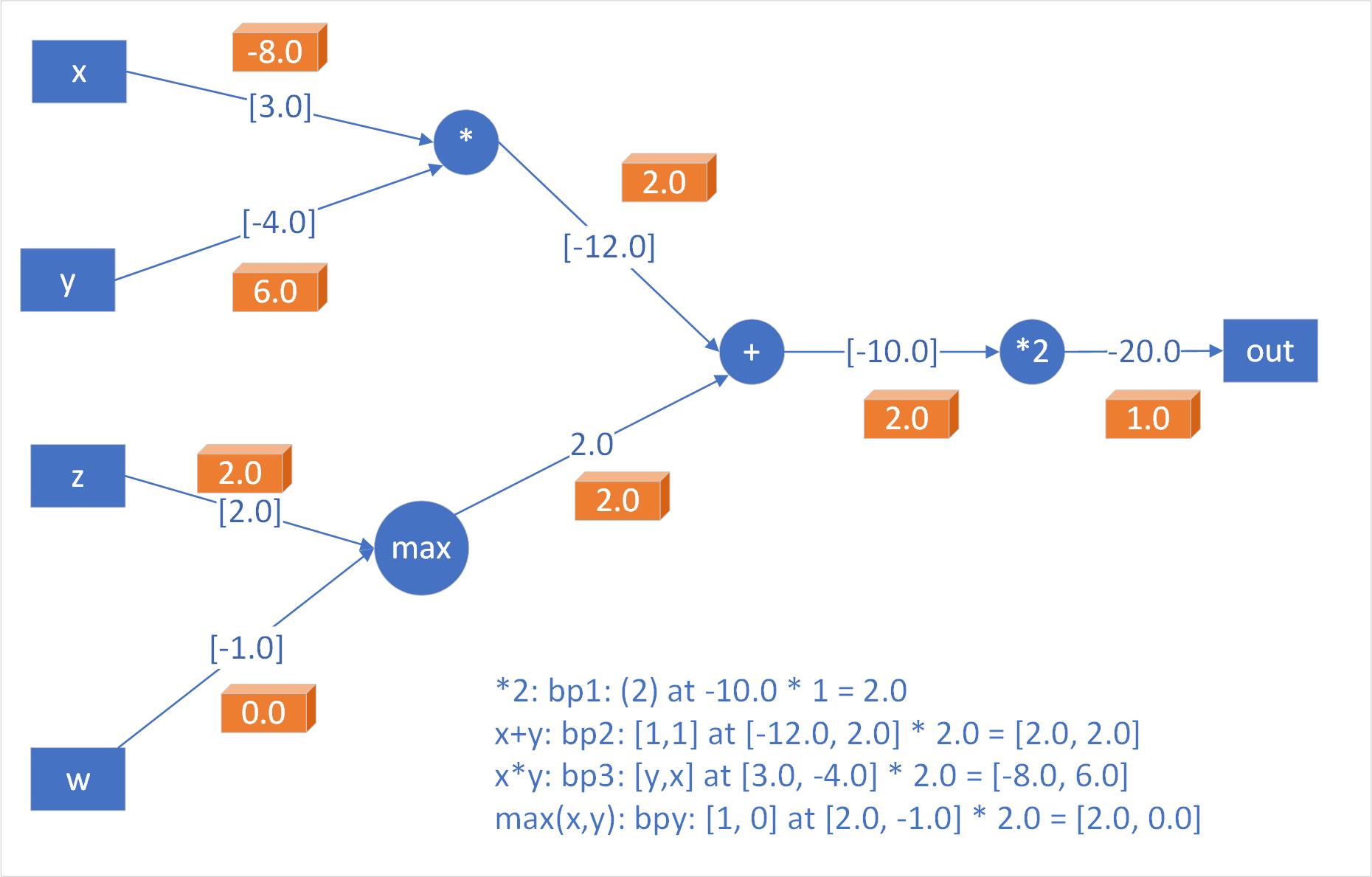
• $f(x, y, z) = (x+y)z$
  • $q = x+y $ and $f = qz$
  • $\frac{\delta f}{\delta q} = z ~and~ \frac{\delta f}{\delta z} = q$
  • $\frac{\delta q}{\delta x} = 1 ~and~ \frac{\delta q}{\delta y} = 1$
• Chain Rule for $\frac{\delta f}{\delta x},~\frac{\delta f}{\delta y}, \frac{\delta f}{\delta z} $
  • $\frac{\delta f}{\delta x} = \frac{\delta f}{\delta q} . \frac{\delta q}{\delta x} $, $\frac{\delta f}{\delta y} = \frac{\delta f}{\delta q} . \frac{\delta q}{\delta y} $, $\frac{\delta f}{\delta z} = \frac{\delta f}{\delta q} . \frac{\delta q}{\delta z} $
  • $[\frac{\delta f}{\delta x},~\frac{\delta f}{\delta y}, \frac{\delta f}{\delta z}]$ tells the sensitivity of $x,y,z$ on $f$.
  • $x=-2, y=5, z=-4 \implies q=3, z=-4 \implies f=-12$
  • For unit change at the output at the final output $f=qz$, the gradient $[dq, dz] = [z, q] = [-4, 3]$
  • Now for $q=x+y$, learns that gradient for its output was $dq=-4$, now $q=x+y$ computes local ingradients $[dx, dy] = [1, 1]$. Thus, $q$ multiplies $dq=-4$ with the local gradients i.e. $[dq.dx, dq.dy] = [1-4, 1-4] = [-4, -4]$
  • $[dx, dy, dz] = [-4, -4, 3]$ is the sensitivity on f
  • Now, if $x, y$ were to decrease due to negative gradient, then the output of node $q$ will increase, which in turn will increase $f$.
    • Backpropogation can be considered as gates communicating to each other through gradient signal, whether they want their outputs to increase or decrease and how strongly, so as to make the final output value higher.

Modularity: Sigmoid

• $f(w, x) = \frac{1}{1+e^{-({w_0x_0+w_1x_1+w_2})}}$
• $f(w, x)$ is a two-dimensional neuron with inputs $x$ and weights $w$ that use the sigmoid activation function.
• $f(w, x)$ is made of multiple gates:
  • $f(x)=\frac{1}{x} \implies dx=\frac{-1}{x^2}$
  • $f_c(x)=c+x \implies dx=1$
  • $f(x)=e^x \implies dx=e^x$
  • $f_a(x)=ax \implies dx=a$
  • $f_c = c+x$ translate by $c$ and $f_a=ax$ scales by $a$

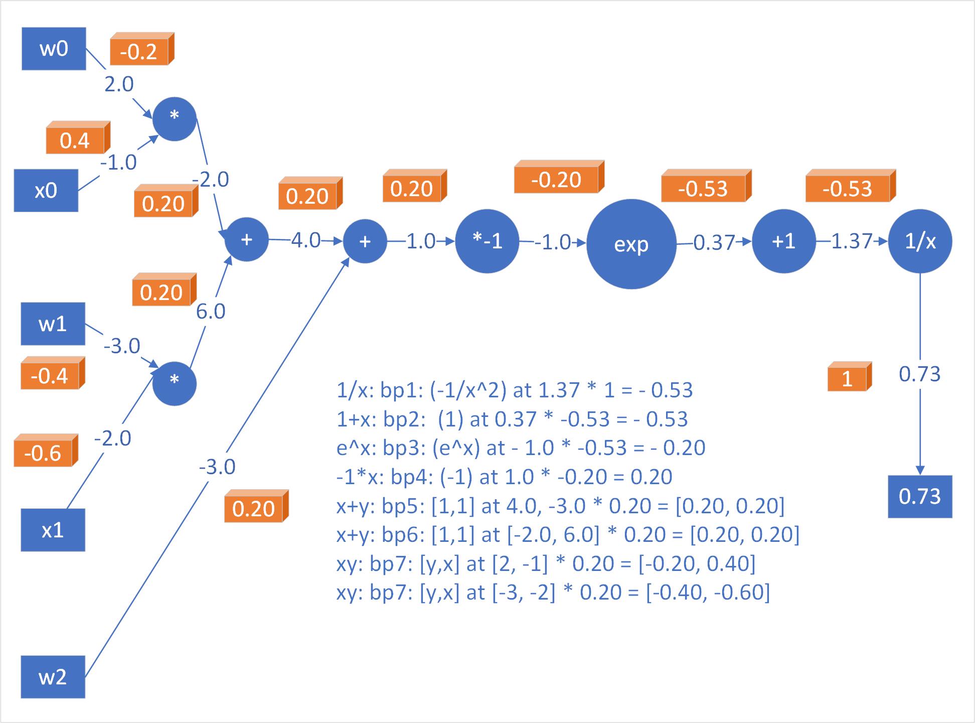
Inputs: $[x_0, x_1]$ = $[-1.0, -2.0]$

Weights: $[w_0, w_1, w_2]$ = $[2.0, -3.0, -3.0]$

Neuron computes dot product and then activation is softly squashed by Sigmoid to be in range of $0$ to $1$ -> $0.73$

We observed, that derivative of sigmoid function is simple:

$\sigma(x) = \frac{1}{1+e^{-x}}$

$\frac{d\sigma(x)}{dx} = \frac{e^{-x}}{(1+e^{-x})^2} = \left( \frac{1 + e^{-x} - 1}{1 + e^{-x}} \right) \left( \frac{1}{1+e^{-x}} \right) = [1 - \sigma(x)] \sigma(x)$

Now, as above, the product of $w_0x_0+w_1x_1+w_2$ is $1$, thus, sigmoid function receives input $1.0$, and outputs $0.73$ in forward pass.

Now since, $\sigma(x)=0.73$, thus, $\frac{d\sigma(x)}{dx}=(1-0.73)*0.73=0.197=0.20$ as computed above in figure.

import math
w = [2, -3, -3]
x = [-1, -2]

dot = w[0] * x[0] + w[1] * x[1] + w[2]
print('dot', dot) # 1
f = 1.0 / (1 + math.exp(-dot))
print('Sigmoid ', f)  # 0.731

ddot = (1 - f) * f
print('derivative of Sigmoid ', ddot) # 0.196

dx = [xi * ddot for xi in x]
dw = [wi * ddot for wi in w]
print(dx) # [-0.196, -0.393]
print(dw) # [0.393, -0.589, -0.589]
# We have now gradients on the inputs

Staged Backpropoogation

In practice, it is helpful to breakdown the forward pass into stages that are easily backpropped.

We created intermediate variable $dot$ that holds dot product of $w$ and $x$. During backward pass, we coompute ddot and then dw and dx that hold gradients.

Backprop in practice: staged computation

$f(x,y) = \frac{x + \sigma(y)}{\sigma(x) + (x+y)^2}$

import math
def sig(x):
    sig = 1.0 / (1 + math.exp(-x))
    return sig
x = 3
y = -4

sigy = sig(y) 	# 1
nr = x + sigy 	# 2
sigx = sig(x) 	# 3

xpy = x + y 			# 4
xpysqr = xpy ** 2 # 5

dr = sigx + xpysqr 	# 6
invdr = 1.0 / dr 		# 7

f = nr * invdr 	# 8
print(f) # 1.545

#8 f = nr * invdr # inp nr and invdr and out 1
d_nr = invdr
d_invdr = nr

#7 invdr = 1.0 / dr # inp dr and out invdr
d_dr = (-1.0 / dr**2) * d_invdr

# 6 dr = sigx + xpysqr # inp [sigx, xpysqr] and out dr
d_sigx = 1 * d_dr
d_xpysqr = 1 * d_dr

#5 xpysqr = xpy ** 2 # inp xpy and out xpysqr
d_xpy = (2 * xpy) * d_xpysqr

#4 xpy = x + y # inp x,y and out xpy
d_x = 1 * d_xpy
d_y = 1 * d_xpy

#3 sigx = sig(x) # inp x and out is sigx
d_x += ((1-sigx) * sigx) * d_sigx

#2 nr = x + sigy # inp x, sigy and out nr
d_x += 1 * d_nr
d_sigy = 1 * d_nr # d is wrt sigy and not y

#1 sigy = sig(y)  # inp y and out sigy
d_y += ((1 - sigy) * sigy) * d_sigy

• Cache Forward Pass Variables Structure code to cache variables of the forward pass so that these are available during backward pass
• Gradients add up at Forks Multivariate chain rule in calculus states that if a variable branches out to different parts of the circuit, the gradients that flow back will add.

Patterns in Backward Flow

• Add Gate
  • Takes the gradient and distributes it equally to all of its inputs, regardless of their values in forward pass
• Max Gate
  • Distributes the gradient (unchanged) to one of its inputs that had the highest value during forward pass
• Multiply Gate
  • Local gradients are the switched input values and multiplied by the gradient on its output
• Unintutive Effects and consequences
  • If one of the input in multiply gate is small, then multiply gate will assign large gradient to smaller input
  • In linear classifiers, we have dot product of $w^T x_i$, thus scale of the data $x_i$ has effect on magnitude of gradients for the weights.
  • If we multiply all input data examples $x_i$ with $1000$, then the gradient on the weights will be 1000 times larger. We need to lower the learning rate to compensate.

Gradients for Vectorized Operations

• Above concepts from single variable can be extended to matrix and vector operations

• Matrix-Matrix Multiply Gradient

  • can be generalized to matrix-vector and vector-vector

  • import numpy as np
        
    W = np.random.randn(5, 10)
    X = np.random.randn(10, 3)
    D = W.dot(X) # (5,3)
        
    d_D = np.random.randn(*D.shape) # Assumed Gradient (5,3)
        
    d_W = d_D.dot(X.T) # swap multiply (5,3).(3,10) = (5,10)
    d_X = W.T.dot(d_D) # Swap multiply (10,5).(5,3) = (10,3)
        
    # expressions of d_W and d_X are computed so that have similar dimensions as W and X
    

  • Gradients on the weights $d_W$ must be same size as $W$, and must be computed using $X$ and $d_D$

  • Gradients on the weights $d_X$ must be same size as $X$, and must be computed using $W$ and $d_D$

​