Notes on CNN - Architecture
Published:
This post covers CNN Architecture from cs231n.
Introduction
- In linear classification, we computed scores $s=W.x$, where $W$ is a weight matrix and $x$ is an input column vector.
- In case of CIFAR-10, $x$ is a $ [32 * 32 * 3=3072, 1] $ column vector and $W$ is a $ [10, 3072] $ matrix, so that output is a vector of $10$ class scores
- Two Layer example Neural Network would compute $s = W_2 * max(0, W_1 * x)$.
- $W_1$ may be $[100, 3072]$ to create 100-dimensional intermediate vector and then $W_2$ can be $[10,100]$ to get 10-dimensional score e vector
- Function $max(0, _)$ is a non-linearity applied element wise. This thresholds all activations that are below zero to zero.
- Non-linearity is computationally critical, as without this $W_2$ and $W_1$ can be collaposed to a single matrix, making the predicted scores to be a linear function of the input.
- Parameters $W_2$ and $W_1$ are learned using SGD and gradients computed from Backpropogation.
- Three Layer Neural Network can be $s = W_3 * max(0, W_2 * max(0, W_1 * x))$.
- $W_3, W_2, W_1$ are parameters to be learned
- The sizes of intermediate hidden vectors are hyper parameters of the network.
Biological Motivation and Connections
- Biological Model
- Neuron is the basic computation unit of brain.
- Neurons are connected with Synapses
- Neuron receives input signal from its Dendrites and produces output signal along its single Axon.
- The Axon eventually branches out and connects via synapses to dendrites of other neurons.
- Human nervous system has 86 Billion Neurons and these neurons are connected with approximately $10^{14} - 10^{15}$ Synapses.
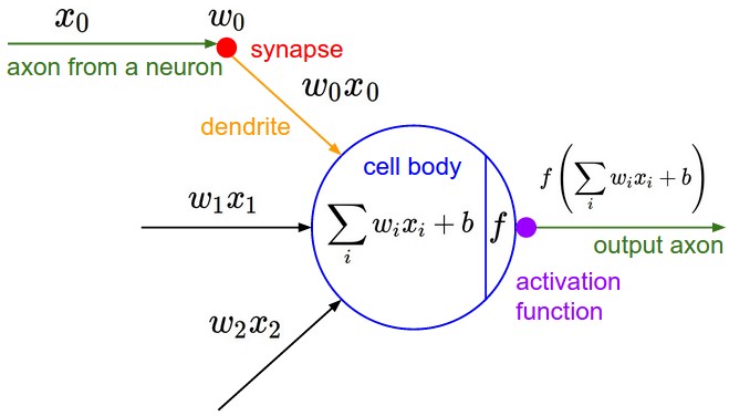
- Computational Model
- Signal $x_0$ that travels along axions interact multiplicately $w_0.x_0$ with dendrites of other neuron based on the synaptic strength $w_0$ at that synapse
- Synaptic strength (weights) are learnable and control the strength of influence and its direction
- Excitory (positive weight) or Inhibitory (negative weight)
https://cs231n.github.io/assets/nn1/neuron_model.jpeg
Basic Model
Dendrites carry signal to the cell body, where they all get summed. Neuron fires if the sum is greater than a threshold, sending a spike along its axon.
We assume that precise timings of the spikes along its axon do not matter, and only frequency of firing communicates information.
We model firing rate with an activation function that represents frequency of the spikes along its axon
class Neuron(object): def forward(self, inputs): cell_body_sum = np.sum(inputs * self.weights) + self.bias firing_rate = 1.0 / (1.0 + math.exp(-cell_body_sum)) # sigmoid return firing_rate- Thus, each neuron performs a dot product with inputs and weights, adds bias and applies non-linearity (activation function)
Coarse Model
- Computational model of biological neuron is very coarse
- There are different types of neurons and each with different types of properties
- Dendrites in biological neurons perform complex non-linear computations
- Exact timing of the output spikes in many systems is known to be important.
Single Neuron as a Linear Classifier
- We can turn single neuron to linear classifier with an appropriate loss function on its output
Binary Softmax Classifier
- We can interpret $\sigma \sum\limits_{i}(w_i . x_i+b)$ to be probability of one of the classes e.g. $ P(y_i=1) \mid x_i,w $
- The probability of other class will be $1-P(y_i=1)$
- We can formulate Cross Entropy Loss
- This will give us binary Softmax classifier (or Logistic Regression).
- Predictions of the classifier are based on whether the output of neuron is greater than $0.5$.
Binary SVM Classifier
- We may attach a max-margin hinge loss to the ouput of neuron and train it to become a binary SVM
Regularization Interpretation
- Regularization loss in biological view can be interpreted as gradual forgetting
Common Activation Functions
- Each activation (non-linear) takes a single number and apply fixed mathematical operation on it.
Sigmoid
- $\sigma(x) = \frac{1}{1+e^{-x}}$
- Sigmoid takes real valued number and squashes in range of $[0,1]$
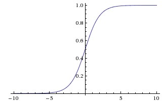
- Sigmoid has nice interpretation as the firing rate:
- value 0 - not firing at all
- value 1 - fully-saturated firing
- Sigmoid is now rarely used due to following drawbacks:
- Sigmoid Saturate and Kill Gradients
- Gradient at the regions where sigmoid saturates become zero
- During backpropogation, local gradients which have become zero will be multiplied with gradient of the output, and this kills the gradient and thus no signal will flow through the neuron to weights and to the data
- We also need to be cautious in initializing the weights of sigmoid neurons to prevent saturation.
- Sigmoid outputs are not zero-centered
- This is not desirable as it can be mitigated by batch processing.
- Neurons in later layers will be receiving data that is not zero-centered. This has implications on the Gradient Descent since the data to neurons is always positive.
- Further, gradients on the weights during backpropogation will be either positive or negative depeding on the whole expression. This may introduce zig-zagging in gradient updates
- However, as gradients are added across batch of data, teh final update for the weights can have variable signs, somewhat mitigating this issue
- Sigmoid Saturate and Kill Gradients
Tanh
- It squashes a real number to the range $[-1, 1]$. Tanh also saturates but have zero-centered output.
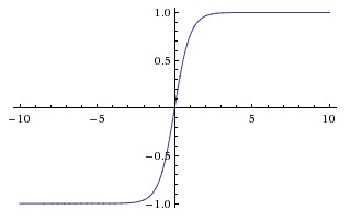
- Tanh nonlinearity is always preferred to the sigmoid nonlinearity
- Tanh neuron is a scaled sigmoid neuron $tanh(x) = 2\sigma(2x)-1$
ReLU
Rectified Linear Unit has become very popular, $f(x)=max(0,x)$
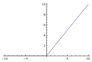
(+) ReLU was found to accelerate by Krizhevsky et al. in factor of 6. This is due to its linear and non-saturating form.
(+) ReLU is easy to implement by thresholding a matrix of activations at zero in comparison to expensive operations like exponential
(-) ReLU can be fragile during training and can die.
- Large gradient flowing through ReLU neuron could cause weight update in such a way that neuron will never activate on any datapoint again.
- ReLU units can irreversibly die during the training since they can get knocked off the data manifold.
- However, with propoer setting of the learning rate this is less frequently an issue.
Leaky ReLU
- Leaky ReLU fix dying ReLU
- Instead of function being zero when $x<0$, a leaky ReLU will have a small negative slope (0.01 or so)
- Variants:
- Leaky ReLU:
- $f(x)= 0.01x$ for $x<0$ and $f(x)=x$ for $x>=0$
- Parametric ReLU (PReLU):
- $f(\alpha, x)=\alpha x$ for $x<0$ and $f(x)=x$ for $x>=0$
- Results are not consistent
- Leaky ReLU:
Maxout
- Maxout by Goodfellow et al. generalizes the ReLU and its leaky version.
- $f(x) = max(w_1^T.x+b_1,~w_2^T.x+b_2)$
- It is a piecewise linear function that returns the maximum of the inputs, designed to be used in conjunction with the dropout regularization technique.
Neural Network Architectures
- Modeled as Neurons connected in an acyclic graph.
- Neural network models are organized into dictinct layers of neurons.
- In a fully connected or dense layer, the neurons between two adjacent layers are fully pairwise connected.
- In a single-layer network, there is no hidden layer e.g. Logistic Regression or SVMs are special case of single-layer artificial neural network or Multi-Layer Perceptron - directly connecting inputs to outputs without hidden layer
- Output Layer:
- Mostly no activation
- represent class scores (in classification) or real-valued target (in regression)
Example Feed-forward Computation
- Repeated Matrix Multiplications interwoven with activation function
- NN is organized into layers so as to make it simple to use matrix and vector operations
- Connections strength for a layer is stored in a matrix
- Modern Convolutional Networks contain millions of parameters and many layers deep.
- Recent Models
- Largest GPT-3 Language model has 175 Billion parameters
- ImageGPT has 6.8 Billion Parameters
Two Layer example network
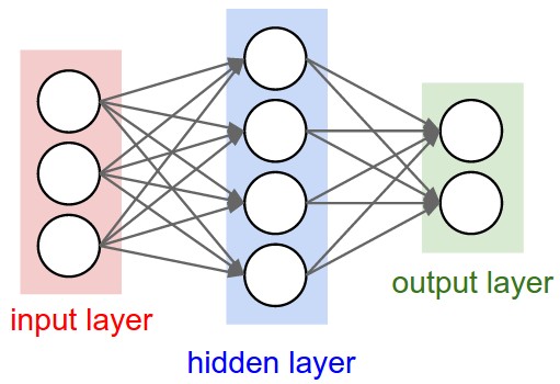
https://cs231n.github.io/assets/nn1/neural_net.jpeg
Input = 3, Hidden=4, Output=2
Two-Layer Network [Hidden and Output]
6 Neurons [4 + 2 ]
$26$ Parameters (Weights and Biases), 3x4+4 +4x2+2
import numpy as np

f = lambda x: 1.0/(1.0 + np.exp(-x))

# input 3
x = np.random.randn(3,1)

# h1 with 4 Neurons
w1 = np.random.randn(4,3)
b1 = np.random.randn(4,1)
h1 = f(np.dot(w1, x) + b1)  # (4,1)

# out with 2 Neuron
w2 = np.random.randn(2,4)
b2 = np.random.randn(2,1)
out = f(np.dot(w2, h1) + b2)  # (1,1)

params = w1.shape[0]*w1.shape[1] + b1.shape[0] + w2.shape[0]*w2.shape[1] + b2.shape[0]

print(params) # 26
print(out.shape) # (2,1)
Every single Neuron has its weights in a row of $W$
Three Layer example network
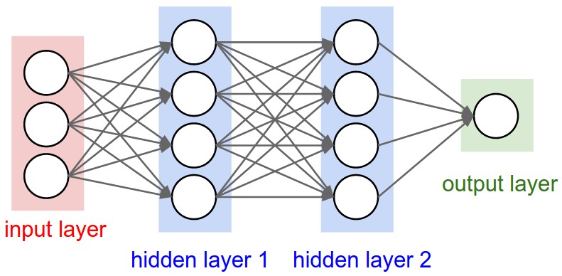
https://cs231n.github.io/assets/nn1/neural_net2.jpeg
Input = 3, Hidden=4, Hidden=4, Output=1
Three-Layer Network [Hidden, Hidden, Output]
9 Neurons [4 + 4 + 1 ]
$41$ Parameters (Weights and Biases), 3x4+4 +4x4+4 + 4x1+1
- Input is [3x1] vector
- Weights $W1$ is [4x3] matrix; and Bias $B1$ is [4x1]
- Weights $W2$ is [4x4] matrix; and Bias $B2$ is [4x1]
- Weights $W3$ is [1x4] matrix; and Bias $B3$ is [1x1]
- $np.dot(W1,x)$ computes activations of all neurons in that layer
Full forward pass of 3-layer neural network is three matrix multiplication with activation functions
import numpy as np

f = lambda x: 1.0/(1.0 + np.exp(-x))

# Input
x = np.random.randn(3,1)

# h1 with 4 Neurons
w1 = np.random.randn(4,3)
b1 = np.random.randn(4,1)
h1 = f(np.dot(w1, x) + b1)  # (4,1)

# h2 with 4 Neurons
w2 = np.random.randn(4,4)
b2 = np.random.randn(4,1)
h2 = f(np.dot(w2, h1) + b2)  # (4,1)

# out with 1 Neuron
w3 = np.random.randn(1,4)
b3 = np.random.randn(1,1)
out = f(np.dot(w3, h2) + b3)  # (1,1)

params = w1.shape[0]*w1.shape[1] + b1.shape[0] + w2.shape[0]*w2.shape[1] + b2.shape[0] + w3.shape[0]*w3.shape[1] + b3.shape[0]

print(params) # 41
print(out.shape) # (1,1)
Input Batch
$x$, instead of one column vector, can hold an entire batch of training data, thus, $x$ can be of shape [-1, n] or [batch_size, n]
Forward pass of a fully connected layer corresponds to one matrix multiplication followed by a bias offset and an activation function
Representational Power
- Neural Network with at least one hidden layer are universal approximators
Given any continuous function $f(x)$ and some $\epsilon > 0$, there exists a Neural Network $g(x)$ with one hidden layer, with a reasonable choice of non-linearity e.g. sigmoid, such that $ f(x)-g(x) <\epsilon~\forall x$
Universality Theorem
- Neural netwoork can approximate any continuous function.
- Two Caveats
- First caveat is not exact but approximate as good as we want
- By increasing number of hidden neurons, we can improve approximation
- Second caveat is that class of functions that can be approximate are the continuous functions.
- Functions with sudden, sharp jumps may not be possible in general to approximate using neural network
- However, continuous approximation of a discontinious function is good enough to use a neural network. Thus, it is not an important limitation
- First caveat is not exact but approximate as good as we want
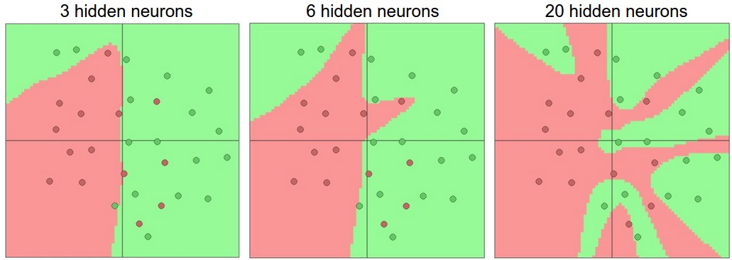
Setting number of layers and their sizes
 https://cs231n.github.io/assets/nn1/layer_sizes.jpeg
High number of neurons can fit the entire training data but may overfit, while the model with low number of neurons (3) can better generalize on the test data set
However, we use other ways to reduce overfitting like L2 regularization, dropout etc to reduce overfitting.
Smaller networks are harder to train with local methods like Gradient Descent.
- Loss function of smaller network have few local minimas and mnay of these minimas are easier to converge to and they are bad i.e. with high loss.
- Bigger neural network contain more local minima and these minima turn out to be much better in terms of their actual loss
Neural Networks are non-convex, so it is hard too study the properties mathematically
Loss in a small network can display a good amount of variance, in some cases it may converge to a good place but in others may get trapped in bad minima
Loss in large network will show low amount of variance, there may be many different solutions. All solutions may be equally good and rely less on the luck of random initialization
Regularization strength is the preferred way to control overfitting the neural network
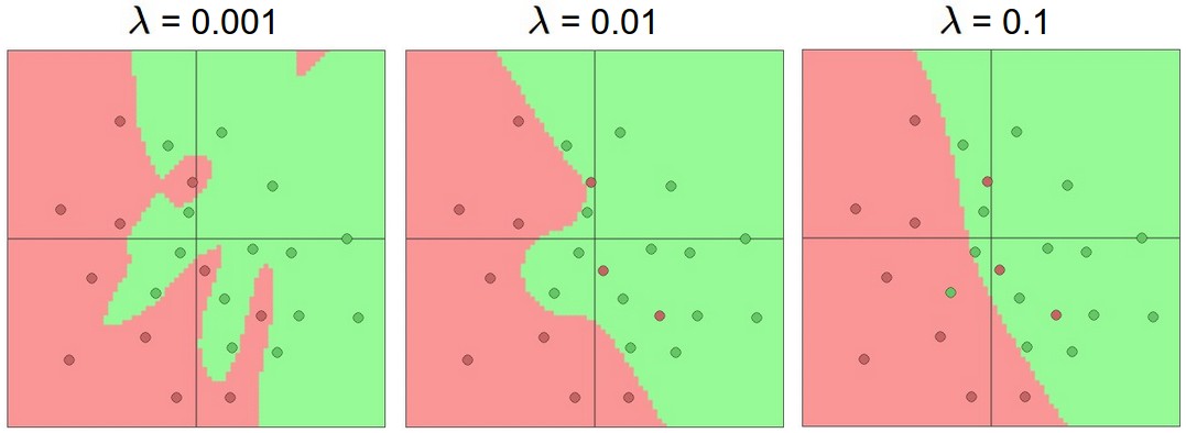
https://cs231n.github.io/assets/nn1/reg_strengths.jpeg


