Probability Distributions
Published:
This post covers Probability Distributions.
Random Variables
- a variable that takes different values determined by chance
- a variable that varies at random
- Notation: $ X $ for variable and $ x $ for value of the variable
- e.g. no of heads in n flips of a fair coin, $ X=0, 1, 2, or~3 $ if $n=3$
- Discrete
- when a random variable can assume only a countable (sometimes infinite) number of values
- Continuous
- when a random variable can assume an uncountable number of values in a line interval
Probability Functions
- a function that provides probabilities for the possible outcomes of a random variable
- Notation: $ f(x) $
- Probability Mass Function (PMF)
- Probability Function for Discrete Random Variable
- $ f(x) = P(X=x) $
- Properties
- $ f(x)>0~~if ~x \in \text{Sample~Space}~else ~0 $
- $ \Sigma_x f(x) = 1 $
- Probability Density Function (PDF)
- Probability Function for Continuous Random Variable
$ f(x) \ne P(X=x) $ since $ P(X=x) = 0 $ for continuous
Thus, we find the probability in interval $ (a,b) $ i.e. $ P(a<X<b) $
Example, https://online.stat.psu.edu/stat414/lesson/14/14.1
A Fast-food chain advertises a burger as weighing a quarter-pound (0.25 pounds). What is the probability that a randomly selected burger weighs between 0.20 and 0.30 pounds i.e. $ P(0.20<X<0.30) $
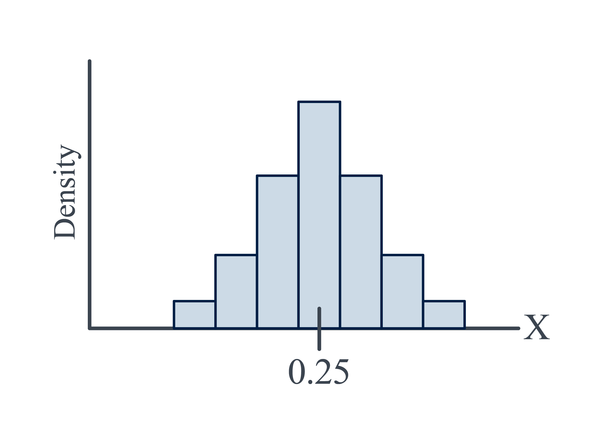
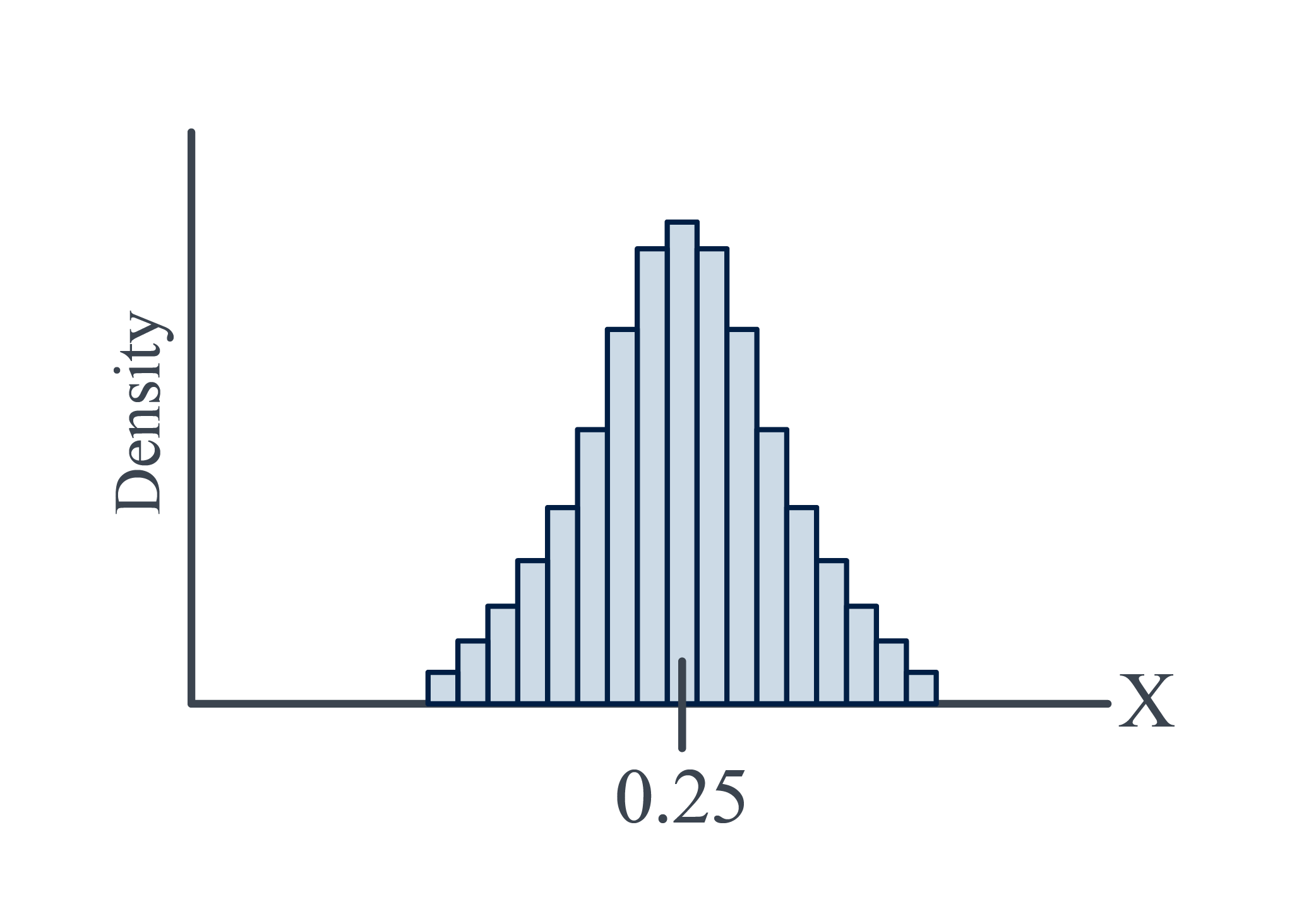
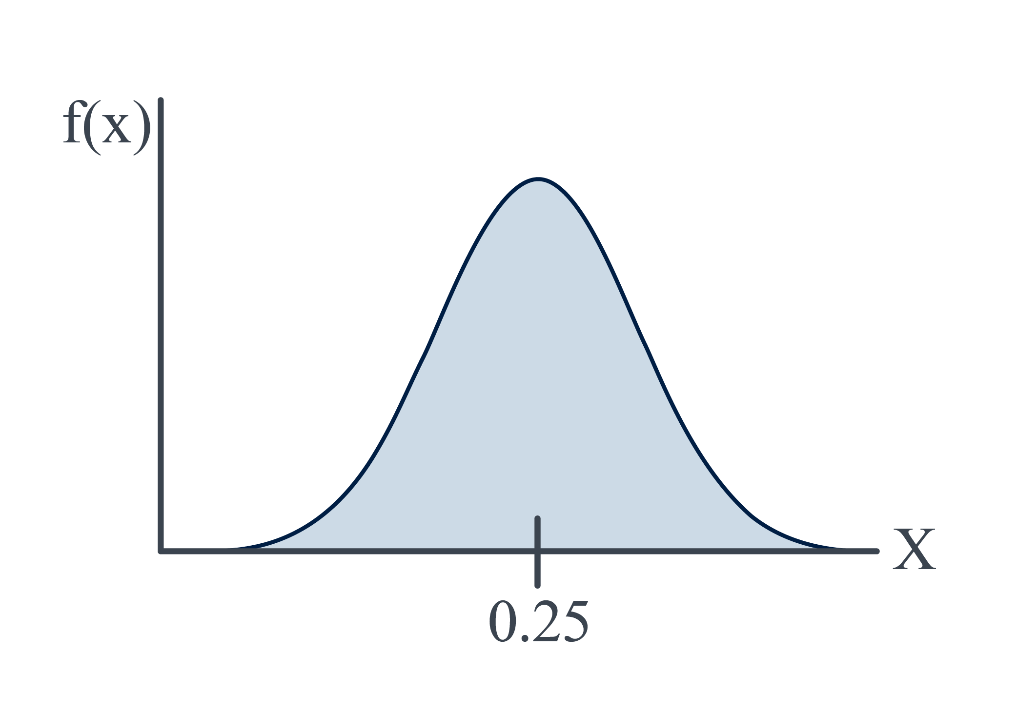
Probability Density Function Total Area is one since the area of each rectangle equals the relative frequency of the corresponding class

Properties
- $ f(x)>0~~if ~x \in \text{Sample Space}~else ~0 $
- The area under the curve is $ 1 $ i.e. $ \int_S f(x)dx=1 $
- Probability that $ x $ belongs to interval $A$ is $ P(X \in A)=\int_A f(x)dx $
- Cumulative Distribution Function
- a function that gives probability of a random variable, $ X $, is less than or equal to $ x $.
- $ F(x) = P(X \le x) $ for discrete
- $ F(x) = P(X < x) $ for continuous since $ P(X=x) = 0 $ for continuous
- $ P(X=x) = \frac{1}{N} ~or~ 0$
- for continuous variable $ N $ can be large so $ \frac{1}{N} \implies 0 $
Discrete Probability Distributions
Dataset = {0, 1, 2, 3, 4}
$ P(X=2) = \frac{1}{5} $
$ PMF = f(x) = \begin{cases} \frac{1}{5} & x=0, 1, 2, 3, 4 \ 0 & \text{otherwise} \end{cases} $
x 0 1 2 3 4 CDF 1/5 2/5 3/5 4/5 1 Expected Value (or mean) of a Discrete Random Variable
- $ \mu = E[X] = \Sigma x_i.f(x_i) $
- Average weighted by Likelihood
- Example: $ \mu = E[X] = 2 $
Variance of a Discrete Random Variable
- $ \sigma^2 = Var(X) = \Sigma (x_i - \mu)^2.f(x_i) $ or
- $ \sigma^2 = Var(X) = \Sigma x_i ^2.f(x_i) - \mu^2 $
Standard Deviation of a Discrete Random Variable
- $ \sigma = \sqrt{variance} $
- Ex: $ \sigma^2 = 2 $ and $ \sigma=1.4142 $
Binomial Random Variables
- Binary Variable - two possible outcomes
- Random variable can be transformed into a binary variable by defining a “success” and a “failure”
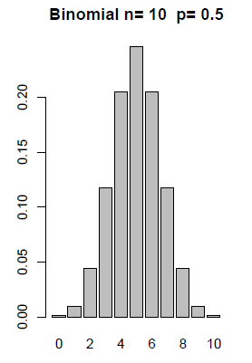
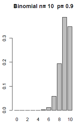
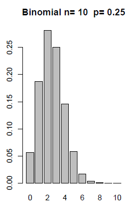
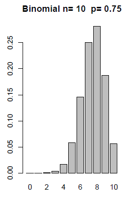
Binomial Distribution
Special Discrete Distribution where there are two distinct complementary outcomes
- Success or Failure
Conditions for Binomial Experiment
- $ n $ identical trials
- Each trial results in success or failure
- Probability of success ($ p $) remains the same from trial to trial
- $ n $ trials are independent i.e. outcome of any trial does not affect the outcome of the others
If above four conditions are satisfied, then random variable $ X $ = number of successes in $ n $ trials is Binomial Random Variable with:
$ \mu = E[X] = np $
$ \sigma^2 = np(1-p) $
$ \sigma = \sqrt{np(1-p)} $
$ \begin{aligned} PMF = f(x) = P(X=x) &= \binom{N}{x} p^x(1-p)^{n-x} \ &= \frac{n!}{x!(n-x)!}p^x(1-p)^{n-x} \end{aligned}$ for $ x=0,1,2,…,n $
%matplotlib inline

from math import comb
import matplotlib.pyplot as plt

def plot_pmf(n, p):
    PMF = [comb(n, x)* p**x * (1-p)**(n-x) for x in range(n+1) ]
    assert sum(PMF) == 1
    plt.bar(x=range(n+1), height=PMF);
    plt.title(f'n={n} p={p}', fontsize=14)
    plt.xlabel('x', fontsize=14)
    plt.ylabel('PMF', fontsize=14)
    plt.show()

plot_pmf(n=10, p=0.1)

plot_pmf(n=10, p=0.25)

plot_pmf(n=10, p=0.5)

plot_pmf(n=10, p=0.75)

plot_pmf(n=10, p=0.9)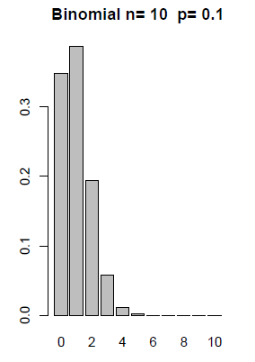
Continuous Probability Distributions
- Examples:
- the amount of rainfall in inches in a year for a city.
- the weight of a newborn baby.
- the height of a randomly selected student.
- Properties
- Define Probability Distribution Function (PDF) of $ X $ as $ f(x) $ where $ P(a<X<b) $ is the area under f(y) over interval from $a~to~b$
- $ P(a< X <b)=\int_a^b f(x)dx $
- Expected Value of Continuous Random Variable
- $ E[X] = \int_a^b xf(x)dx $ for continuous random variable $X$ in range $(a,b)$
- $f(x)$ is probability density with units prob/(unit of X)
- $f(x)dx$ is the probability that $X$ is in an infinitesimal range of width $dx$ around $x$
- Variance of Continuous Random Variable
- $ \sigma^2 = E[(X-\mu)^2] $ or
- $ \sigma^2 = E[X^2] -\mu^2] $
- References