This post covers Normal Distribution from https://www.mathsisfun.com/data/standard-normal-distribution.html and https://www.mathsisfun.com/data/standard-deviation.html

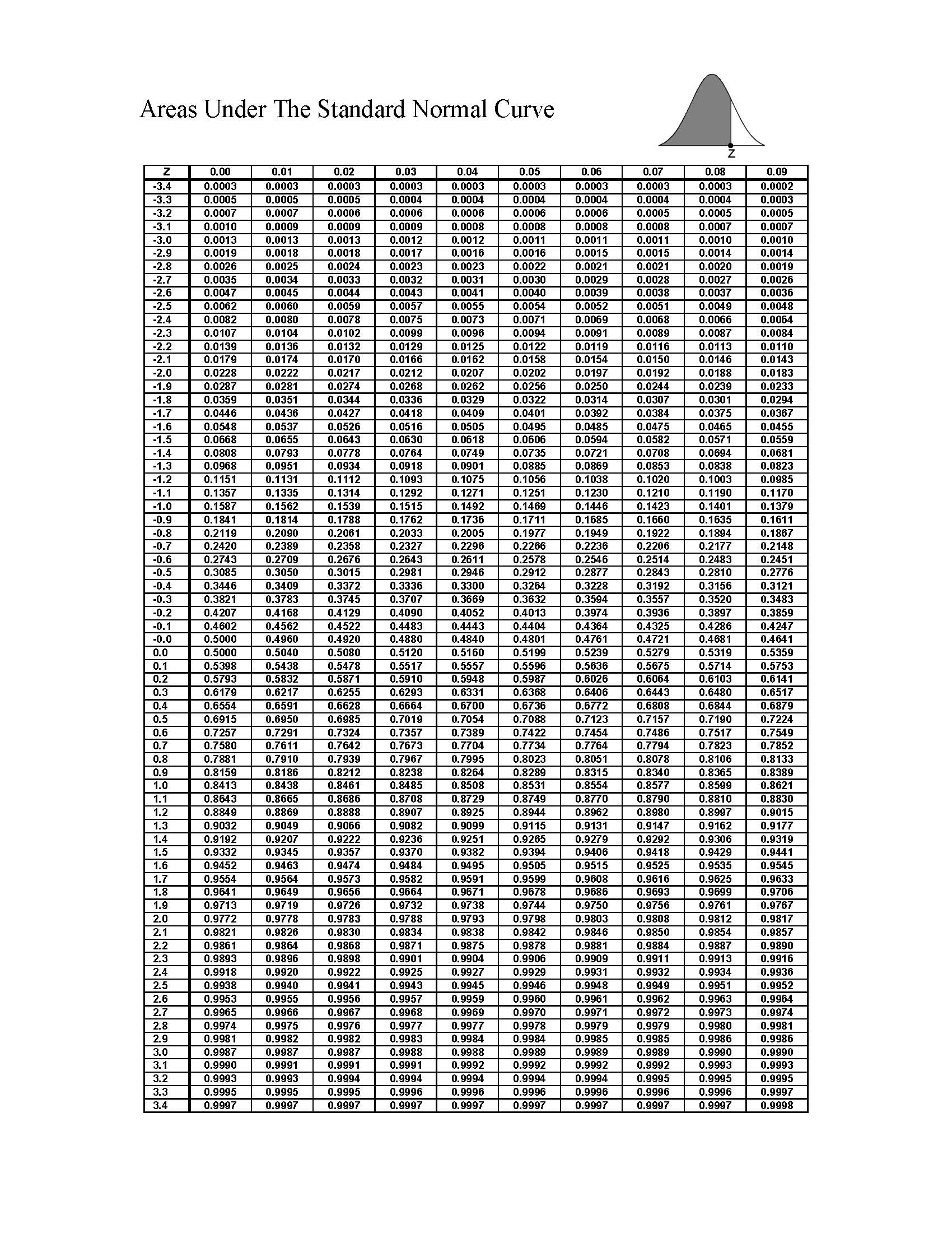
Ztable: https://www.mathsisfun.com/data/standard-normal-distribution-table.html

Ztable: Z

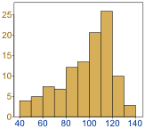
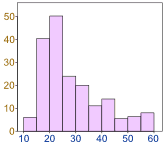
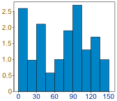
Data Distribution

Spread more on left	Spread more on right	jumbled up	Data around central value

• Examples of Normal Distribution

  • Heights of people
  • size of things produced by machines
  • errors in measurements
  • blood pressure
  • marks on a test

Normal Distribution

• mean = median = mode
• symmetry about the center
• 50% of values less than the mean and 50% greater than the mean

Standard Deviation

• measure of how spread out numbers are
• square root of the Variance

• Variance is average of the squared differences from the Mean

• Example
• 
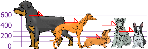
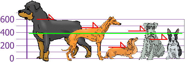
• Heights: 600mm, 470mm, 170mm, 430mm and 300mm
• Compute Mean, the Variance, and the Standard Deviation
• Mean
  • 394
  • 
• Variance
  • Each Dog’s Difference from the mean
  • 
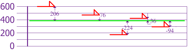
  • 21704
• Standard Deviation
  • 147.32
  • 
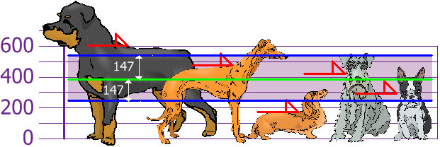
  • SD is useful since we can show which heights are within one Standard Deviation (147) of the mean (394 mm)
  • Using Standard Deviation, we have a standard way of knowing what is normal and what is extra large, or extra small
• Correction for Sample Data
  • If the data is population, then variance is average of squared differences
  • If the data is sample from a bigger population, we divide by N-1 for calculating variance
  • Sample Variance: 27130
  • Sample Standard Deviation: 165

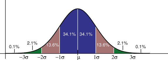
Standard Deviations

68% of values are within 1 standard deviation of the mean / 95% of values are within 2 standard deviation of the mean / 99.7% of values are within 3 standard deviation of the mean

• Example

  • 95% of students are between 1.1m and 1.7m tall. Assume data is normally distributed, compute mean and standard deviation

  • Mean is halfway between 1.1m and 1.7m
    • Mean = (1.1m + 1.7m) / 2 = 1.4m
  • 95% is 2 standard deviations either side of the mean (a total of 4 standard deviations) so:
    • $1~SD = \frac{1.7m-1.1m}{4}=0.15$

  • Result

    

It is good to know the standard deviation, because we can say that any value is:

• likely to be within 1 standard deviation (68 out of 100 should be)
• very likely to be within 2 standard deviations (95 out of 100 should be)
• almost certainly within 3 standard deviations (997 out of 1000 should be)

Standard Scores

• The number of standard deviations from the mean is also called

  • Standard Score
  • sigma
  • z-score

• Example

  • One student is 1.85m tall

    • Is there a standard way of telling information about height

    

  • 1.85m is 3 standard deviations from the mean of 1.4
    • $ \frac{1.85 - 1.4}{.15} = \frac{.45}{.15}=3 $
  • Thus, z-score is 3.0

• 

• Example: Travel Time

  • 26, 33, 65, 28, 34, 55, 25, 44, 50, 36, 26, 37, 43, 62, 35, 38, 45, 32, 28, 34

  • Mean is 38.8 minutes, and the Standard Deviation is 11.4 minutes

  • Compute z-scores

    • $z = \frac{x - \mu}{\sigma}$
    • $z = \frac{x - mean}{std}$

      data = np.array([26, 33, 65, 28, 34, 55, 25, 44, 50, 36, 26, 37, 43, 62, 35, 38, 45, 32, 28, 34])
          
      mean = np.mean(data)
      std = np.std(data)
          
      z = (data - mean)/std # stats.zscore(data)
      print(z)
          
      z1 = data[np.where(np.abs(z)>1)]
      z2 = data[np.where(np.abs(z)>2)]
      z3 = data[np.where(np.abs(z)>3)]
          
      print(z1)
      print(z2)
      print(z3)
    

• Why Standardize?

  • Marks out of 60
    • 20, 15, 26, 32, 18, 28, 35, 14, 26, 22, 17
    • Most student have less than 30 marks
  • Mean = 23 and Standard Deviation = 6.6
  • -0.45, -1.21, 0.45, 1.36, -0.76, 0.76, 1.82, -1.36, 0.45, -0.15, -0.91
    • Only two students have lower marks than one SD

• Your score in a recent test was 0.5 standard deviations above the average, how many people scored lower than you did?
  • Between 0 and 0.5 is 19.1%
  • Less than 0 is 50% (left half of the curve)
  • So the total less than you is:
    • 50% + 19.1% = 69.1%

References

• https://www.mathsisfun.com/data/standard-normal-distribution.html
• https://www.statisticshowto.com/probability-and-statistics/normal-distributions/