Hypothesis
Published:
This post covers Hypothesis Testing.
Hypothesis Testing
| Dependent Variable (Measured in scale from 1 to 10) | Sample Mean $\bar{X}$ (n=20) | Probability | Likely or Unlikely |
|---|---|---|---|
| Student Engagement | $\bar{X}_E = $ Something | $ p \sim 0.05 $ | |
| Student Learning | $\bar{X}_L =$ Something | $ p \sim 0.10 $ |
- Threshold is difficult to decide - likely or unlikely
|  |
|  |
|  | | ———————————– | ———————————————————— | ———————————————————— |
$\alpha$ Levels of Likelihood (unlikelihood) - One Tailed
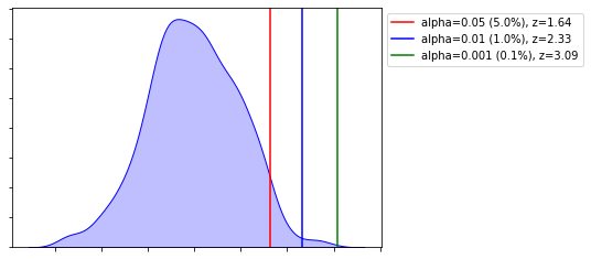
- If the probability of getting a sample mean is less than
- $ \alpha = 0.05 (5\%)$
- $ \alpha = 0.01 (1\%)$
- $ \alpha = 0.001 (0.1\%)$
- then it is considered unlikely.
- If the probability of getting a particular sample mean is less than $\alpha$ (0.05, 0.01, 0.001), it is unlikely to occur
- If a sample mean has a z-score greater than $z^*$ (1.64, 2.33, 3.09), it is unlikely to occur
Z-Critical Value
If the probability of obtaining a particular sample mean is less than the alpha level.
- Then it will fall in the tail which is called the Critical Region and Z-value is called the z-critical value
If the z-score of a sample mean is greater than z-critical value, we have evidence that these sample statistics are different from the regular or untreated population.
If the probability of critical region = alpha level = 0.05
z-critical value = 1.64
alpha = 5/100
z = stats.norm.ppf(1 - alpha)
label = f'alpha={alpha} ({alpha*100}%), z={z:.2f}'
If the probability of critical region = alpha level = 0.01
z-critical value = 2.33
alpha = 1/100
z = stats.norm.ppf(1 - alpha)
label = f'alpha={alpha} ({alpha*100}%), z={z:.2f}'
If the probability of critical region = alpha level = 0.001
z-critical value = 3.09
alpha = 0.1/100
z = stats.norm.ppf(1 - alpha)
label = f'alpha={alpha} ({alpha*100}%), z={z:.2f}'
Example
- Sample Mean = $\bar{X}$
- $z = \frac{\bar{X}-\mu}{\frac{\sigma}{\sqrt{n}}}$
- Let $z=1.82$
- $\bar{X}$ is significant at $p<0.05$
- since zcr > 1.64 (0.05) and < 2.33 (0.01)
- Red region
Example
z-score Significant at: ( p< ) 3.14 0.001 2.07 0.05 2.57 0.01 14.31 0.001
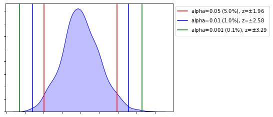
Two-Tailed Critical Values
- Split the Alpha Level in half
Hypothesis

| One Tailed Test | One Tailed Test | Two Tailed Test |
|---|---|---|
 |  |  |
Two Outcomes
- Sample Mean is outside the Critical Region
- Sample Mean is inside the Critical Region
$H_0$, Null Hypothesis
- No Significant difference between the current population parameters and what will be the new population parameters after the intervention
- Sample Mean lies outside the critical region
- $\mu \sim \mu_I$
$H_a$ or $H_1$, Alternate Hypothesis
- $\mu < \mu_I$
- $\mu > \mu_I$
- $\mu \ne \mu_I$
|  |
| | | | ———————————————————— | ———————————————————— | —- |
Example
- $H_0$: Most dogs have four legs (most = more than 50%)
- $H_A$: Most dogs have less than four dogs
- Sample 10 dogs and find all have four legs
- Did we prove that Null Hypothesis is True?
- No
- We have evidence to suggest that most dogs have four legs - since we have sample - but we didn’t prove - we also didn’t prove alternative hypothesis
- We simply fail to reject the Null Hypothesis
- No
- Did we prove that Null Hypothesis is True?
- Sample 10 dogs and find that 6 dogs have 3 legs
- Is this evidence to reject the null hypothesis that most dogs have 4 legs
- Yes
- Based on the sample, reject Null in favor of Alternative
| Z | $\alpha$-Level | Test |
|---|---|---|
| $\pm 1.64$ | 5% or 0.05 | One-tail |
| $\pm 2.33$ | 1% or 0.01 | One-tail |
| $\pm 3.09$ | 0.1% or 0.001 | One-tail |
| $\pm 1.96$ | 5% or 0.05 | Two-tail |
| $\pm 2.58$ | 1% or 0.01 | Two-tail |
| $\pm 3.29$ | 0.1% or 0.001 | Two-tail |
Example
EngagementLearning.csv
$\mu = 7.47, \sigma = 2.413$
Hypothesis Test
- $H_0$ - no significant difference
- not make learners more engaged
- results in the same level of engagement
- $H_1$ - significant difference
- Make Learners more Engaged, $\mu < \mu_I$
- Make Learners less Engaged, $\mu > \mu_I$
- Change how much learners are engaged, $\mu \ne \mu_I$
- $H_0$ - no significant difference
Which Hypothesis Test to choose
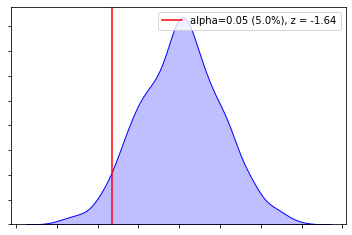
- $\mu < \mu_I$ - One-Tailed Test (cr - right)
- $\mu > \mu_I$ - One-Tailed Test (cr - left)
- $\mu \ne \mu_I$ - Two-Tailed Test
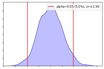
Two-Tailed Test on Learning at 5 % Level
z-critical values, $\pm 1.96$
lb = round(stats.norm.ppf(0.025), 3) # -1.96
ub = round(stats.norm.ppf(0.025+.95), 3) # 1.96
- Example - Learning Engagement
- Population
- $\mu = 7.47, \sigma = 2.413$
- Hypothesis
- $H_0 = \mu = \mu_I$
- $H_A = \mu \ne \mu_I$
- Sample
- $\bar{x} = 8.3,~ n = 30$
- $std_error = \frac{\sigma}{\sqrt(n)} = \frac{2.413}{\sqrt{30}} = 0.441$
- Compute the z-score of the sample mean of the sampling distribution
- $z = \frac{xbar - mu}{std_error} = \frac{8.3 - 7.47}{0.441} = 1.882$
- The sample is not different if it is within $\pm 1.882$
- $p = 0.0301 + 0.0301 = 0.0602 > 0.05$
- Fail to Reject
- Not enough evidence that the new population parameters will not be significantly different than the current
- Population
import scipy.stats
mu = 7.47
sigma = 2.413

n = 30
xbar = 8.3
std_error = sigma / np.sqrt(n)
std_error = round(std_error, 3)

print(f"std_error = sigma / np.sqrt(n) = {std_error}") # 0.441

z = (xbar - mu)/std_error
z = round(z, 3)
print(f"z = {z}") # 1.882

p = round(scipy.stats.norm.sf(z), 3)
p = p * 2 # Two tail
print(f"p = {p}") # 0.06
Decision Errors
| |
 | | ———————————————————— | ———————————————————— |
| Reject $H_0$ | Retain $H_0$ | |
|---|---|---|
| $H_0$ True | Statistical Decision Errors Type I Error | Correct |
| $H_0$ False | Correct | Statistical Decision Errors Type II Error |
Same Example - Learning Engagement (n = 30)
- Population
- $\mu = 7.47, \sigma = 2.413$
- Hypothesis
- $H_0 = \mu = \mu_I$
- $H_A = \mu \ne \mu_I$
- Sample
- $\bar{x} = 8.3,~ n = 30$
- $std_error = \frac{\sigma}{\sqrt(n)} = \frac{2.413}{\sqrt{30}} = 0.441$
- Compute the z-score of the sample mean of the sampling distribution
- $z = \frac{xbar - mu}{std_error} = \frac{8.3 - 7.47}{0.441} = 1.882$
- The sample is not different if it is within $\pm 1.882$
- $p = 0.0301 + 0.0301 = 0.0602 > 0.05$
- Fail to Reject
- Not enough evidence that the new population parameters will not be significantly different than the current
import scipy.stats
mu = 7.47
sigma = 2.413

n = 30
xbar = 8.3
std_error = sigma / np.sqrt(n)
std_error = round(std_error, 3)

print(f"std_error = sigma / np.sqrt(n) = {std_error}") # 0.441

z = (xbar - mu)/std_error
z = round(z, 3)
print(f"z = {z}") # 1.882

p = round(scipy.stats.norm.sf(z), 3)
p = p * 2 # Two tail
print(f"p = {p}") # 0.06
Same Example - Learning Engagement (n = 50)
- Population
- $\mu = 7.47, \sigma = 2.413$
- Hypothesis
- $H_0 = \mu = \mu_I$
- $H_A = \mu \ne \mu_I$
- Sample
- $\bar{x} = 8.3,~ n = 50$
- $std_error = \frac{\sigma}{\sqrt(n)} = \frac{2.413}{\sqrt{50}} = 0.341$
- Compute the z-score of the sample mean of the sampling distribution
- $z = \frac{xbar - mu}{std_error} = \frac{8.3 - 7.47}{0.341} = 2.434$
- The sample is not different if it is within $\pm 2.434$
- $p = 0.0075 + 0.0075 = 0.015 < 0.05$
- Reject the Null
import scipy.stats
mu = 7.47
sigma = 2.413

n = 50
xbar = 8.3
std_error = sigma / np.sqrt(n)
std_error = round(std_error, 3)

print(f"std_error = sigma / np.sqrt(n) = {std_error}") # 0.341

z = (xbar - mu)/std_error
z = round(z, 3)
print(f"z = {z}") # 2.434

p = round(scipy.stats.norm.sf(z), 3)
p = p * 2 # Two tail
print(f"p = {p}") # 0.014
- Type - II error
- Fail to reject the null
- Could be type 2 error
- Fail to reject the null