Estimation
Published:
This post covers Estimation.
- Population Mean = 37.72
- Population Standard Deviation = $\sigma$ = 16.04
- Sample Size = 35
- Sample Mean = 40
- Standard Error = $\frac{\sigma}{\sqrt{n}}$ = $\frac{16.04}{\sqrt{35}} = 2.71$
- What would be the best guess of mean of Population for treated population if we have sample mean 40 and sample size 35
- Point Estimate = 40
- What will be the range of population mean for the treated population if the sample mean is 40
- 68–95–99.7 rule
- Approx 68% of sample means fall within 2.711 of 40
- Approx 95% of sample means fall within 5.423 of 40
- Margin of Error
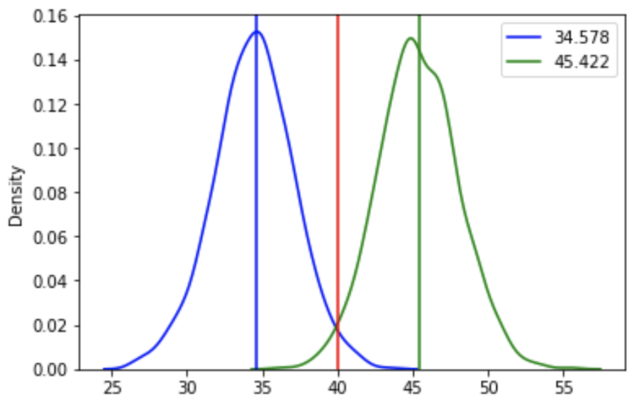
- There is a 95% chance that sample mean 40 will be within 34.577 and 45.423 of the new population mean
- 2*std_error 5.423 is the Margin of Error
- Interval Estimate for Population Mean
- 95% of sample means will be within 2 std deviations 5.423 from the sample mean 40
- Confidence Interval Bounds
- $ \mu - 2 * \frac{\sigma}{\sqrt{n}} < 40 < \mu + 2 * \frac{\sigma}{\sqrt{n}} $
- $ - 2 * \frac{\sigma}{\sqrt{n}} < 40 - \mu < 2 * \frac{\sigma}{\sqrt{n}} $
- $ -40 - 2 * \frac{\sigma}{\sqrt{n}} < - \mu < -40 + 2 * \frac{\sigma}{\sqrt{n}} $
- $ 40 + 2 * \frac{\sigma}{\sqrt{n}} > \mu > 40 - 2 * \frac{\sigma}{\sqrt{n}} $
- $ 40 - 2 * \frac{\sigma}{\sqrt{n}} < \mu < 40 + 2 * \frac{\sigma}{\sqrt{n}} $
- 95% confidence interval for the mean is 34.577, 45.423
- Exact Z-scores
- What are the Z-score values that bound 95% of the data
- Z Score values that bound 95% of the data are -1.96, 1.96
- 95% CI with exact Z-Scores
- 95% of sample means fall within 1.96 standard errors from the population mean
- 95% confidence interval for mean: (34.68644, 45.31356)
- Generalize Point Estimate
- Let $\bar{X}$ be mean of sample and $\mu$ be population mean
- What is point estimate?
- $\bar{X}$
- What is Interval Estimate?
- $\bar{X} - 1.96\frac{\sigma}{\sqrt{n}},~\bar{X} + 1.96\frac{\sigma}{\sqrt{n}}$
- What is point estimate?
- Large Sample Size
- n = 250
- Standard Error = $\frac{\sigma}{\sqrt{n}}$ = $\frac{16.04}{\sqrt{250}} = 1.01 $
- 95% confidence interval for mean: (38.02, 41.98)
- Let $\bar{X}$ be mean of sample and $\mu$ be population mean
- Bigger Sample, Smaller CI
- 95% confidence estimate when n= 35 is (34.6884, 45.3116)
- 95% confidence interval when n=250 is (38.0204, 41.9796)
- Z for 98% CI
- Z Score values that bound 98% of the data are -2.33, 2.33
- 98% confidence interval for mean: (37.6467, 42.3533) for sample size 250
- Critical Values of Z
- $\pm 2.33$ - critical values of Z for 98% CI
- $\pm 1.96$ - critical values of Z for 95% CI

L02 - Estimation
%matplotlib inline

import numpy as np
import pandas as pd
import scipy
import itertools
import math
import matplotlib.pyplot as plt
import seaborn as sns
import random
import os
def get_data(data_file):
    with open(data_file, 'r') as fp:
        data = fp.readlines()

    data = [float(d.strip()) for d in data]
    return data

score_file = './data/Klout/score.csv'
data = get_data(score_file)
print(len(data))
Point Estimate for Population Mean
sample_size = 35
sample_mean = 40
std_error = 2.71

# What would be best guess of mean of population
# for treated population
# if we have sample (n=35, mean=40)
# from previous lesson
point_estimate = sample_mean
print(point_estimate)
%matplotlib inline
import matplotlib.pyplot as plt
import random
import numpy as np

fig, ax1 = plt.subplots()

ax1.hist(data, alpha=0.5);


mean = np.mean(sample),
std_error = np.std(sample)/np.sqrt(len(sample))

for i in range(10):
    sample = random.sample(data, 35)
    mean = np.mean(sample),
    std_error = np.std(sample)/np.sqrt(len(sample))

    values = np.random.normal(loc=mean, scale=std_error, size=1000)

    ax2 = ax1.twinx()
    sns.kdeplot(values, color="red", ax=ax2);
# What will be range of population mean
# for treated population
# if sample mean is 40

msg = f'Approx 68% of sample means fall within {std_error} of {sample_mean}'
print(msg)

msg = f'Approx 95% of sample means fall within {2*std_error} of {sample_mean}'
print(msg)
def plot_sd(mean, se, ax=None, color='blue'):
    values = np.random.normal(loc=mean, scale=se, size=1000) # 1000 values using normal distribution
    if ax:
      	sns.kdeplot(values, ax=ax, color=color);
    else:
	      sns.kdeplot(values, color=color);
Margin of Error
ax = plt.subplot()

plot_sd(sample_mean, std_error, ax=ax)

ax.axvline(sample_mean, color='red',
           label=sample_mean);

x1 = sample_mean - 2*std_error
x2 = sample_mean + 2*std_error

ax.axvline(x1, color='green', label=x1);
ax.axvline(x2, color='blue', label=x2);
plt.legend();


msg = "There is 95% chance that sample mean"
msg += f" {sample_mean} will be within"
msg += f" {x1} and {x2} of new population mean"
print(msg)

msg = f"2*std_error {2*std_error} is"
msg += " Margin of Error"
print(msg)
Interval Estimate for Population Mean
- $ \mu - 2 * \frac{\sigma}{\sqrt{n}},~~\mu + 2 * \frac{\sigma}{\sqrt{n}} $
msg = f"95% of sample means will be within 2 std deviation {2 * std_error} from sample mean {sample_mean}"
print(msg)
Confidence Interval Bounds
- $ \mu - 2 * \frac{\sigma}{\sqrt{n}} < 40 < \mu + 2 * \frac{\sigma}{\sqrt{n}} $
- $ - 2 * \frac{\sigma}{\sqrt{n}} < 40 - \mu < 2 * \frac{\sigma}{\sqrt{n}} $
- $ -40 - 2 * \frac{\sigma}{\sqrt{n}} < - \mu < -40 + 2 * \frac{\sigma}{\sqrt{n}} $
- $ 40 + 2 * \frac{\sigma}{\sqrt{n}} > \mu > 40 - 2 * \frac{\sigma}{\sqrt{n}} $
- $ 40 - 2 * \frac{\sigma}{\sqrt{n}} < \mu < 40 + 2 * \frac{\sigma}{\sqrt{n}} $
print(f'95% confidence interval for the mean is {sample_mean - 2 * std_error}, {sample_mean + 2 * std_error}')
ax = plt.subplot()

plot_sd(sample_mean - 2 * std_error, std_error,
        ax=ax, color='blue')

plot_sd(sample_mean + 2 * std_error, std_error,
        ax=ax, color='green')

ax.axvline(sample_mean - 2 * std_error,
           label=sample_mean - 2 * std_error,
           color='blue');

ax.axvline(sample_mean + 2 * std_error,
           label=sample_mean + 2 * std_error,
           color='green');

ax.axvline(sample_mean, color='red');

plt.legend();
Exact Z-scores
# What are the Z-score values that bound
# 95% of the data
ax = plt.subplot()

sample_mean_ = 0
std_error_ = 1

plot_sd(sample_mean_, std_error_, ax=ax)

ax.axvline(sample_mean_ - 2* std_error_,
           color='red',
           label=sample_mean_ - 2* std_error_);
ax.axvline(sample_mean_ + 2* std_error_,
           color='green',
           label=sample_mean_ + 2* std_error_);

area1 = 2.5/100 # Less that red line
z1 = scipy.stats.norm.ppf(area1)

area2 =  area1 + .95
z2 = scipy.stats.norm.ppf(area2)

msg = f"Z Score values that bound 95%"
msg += f" of the data are {z1:.2f}, {z2:.2f}"

print(msg)
95% CI with exact Z-Scores
- 95% of sample means fall within 1.96 standard errors from the population mean
CI95_lower = sample_mean - 1.96 * std_error
CI95_upper = sample_mean + 1.96 * std_error
CI95 = CI95_lower, CI95_upper

print(f'95% confidence interval for mean: {CI95}')
Generalize Point Estimate
- Let $\bar{X}$ be mean of sample and $\mu$ be population mean
- What is point estimate?
- $\bar{X}$
- What is Interval Estimate?
- $\bar{X} - 1.96\frac{\sigma}{\sqrt{n}},~\bar{X} + 1.96\frac{\sigma}{\sqrt{n}}$
- What is point estimate?
CI Range for Larger Sample Size
- sample_size = 35
- sample_mean = 40
- std_error = 2.71
- 95% confidence estimate is (34.6884, 45.3116)
# What would be best guess of mean of population
# if we have sample (n=35, mean=40)
# from previous lesson

sample_size = 250
sample_mean = 40
std_error = 1.01

CI95_lower = sample_mean - 1.96 * std_error
CI95_upper = sample_mean + 1.96 * std_error
CI95 = CI95_lower, CI95_upper

print(f'95% confidence interval for mean: {CI95}')
Bigger Sample, Smaller CI
- 95% confidence estimate when n= 35 is (34.6884, 45.3116)
- 95% confidence interval when n=250 is (38.0204, 41.9796)
Treatment Effect
- occurs when the intervention affects the population mean
- When the sample mean is far on the tails of the sampling distribution, and therefore unlikely to have occurred by chance, there is evidence for a treatment effect
Z for 98% CI
# What are the Z-score values that bound
# 98% of the data

ax = plt.subplot()

sample_mean_ = 0
std_error_ = 1

plot_sd(sample_mean_, std_error_, ax=ax)

ax.axvline(sample_mean_ - 3* std_error_,
           color='red',
           label=sample_mean_ - 2* std_error_);

ax.axvline(sample_mean_ + 3* std_error_,
           color='green',
           label=sample_mean_ + 2* std_error_);

area1 = 1/100 # Less that red line
z1 = scipy.stats.norm.ppf(area1)

area2 =  area1 + .98
z2 = scipy.stats.norm.ppf(area2)

msg = "Z Score values that bound 98% of the data"
msg += f"are {z1:.2f}, {z2:.2f}"
print(msg)
98% CI
# What would be best guess of mean of population
# if we have sample (n=35, mean=40)
# from previous lesson

sample_size = 250
sample_mean = 40
std_error = 1.01

CI98_lower = sample_mean - 2.33 * std_error
CI98_upper = sample_mean + 2.33 * std_error
CI98 = CI98_lower, CI98_upper

print(f'98% confidence interval for mean: {CI98}')
Critical Values of Z
- $\pm 2.33$ - critical values of Z for 98% CI
- $\pm 1.96$ - critical values of Z for 95% CI
Engagement Ratio
data_file = './data/EngagementRatio/EngagementRatio.csv'
data = get_data(data_file)
n = len(data)
print(n)
# Population Parameters
print(f'Population Mean={np.mean(data):.3f} and Standard Deviation = {np.std(data):.3f}')
# Sample of 20 Students with mean 0.13
sample_size = 20
X_bar = 0.13
# Point Estimate
print(X_bar)
# Interval Estimate
std_error = np.std(data)/np.sqrt(sample_size)
print(f'{std_error:.3f}')

ll = X_bar - 1.96 * std_error
ul = X_bar + 1.96 * std_error

print(f'95% CI Interval Estimate is {ll:.3f}, {ul:.3f}')
msg = f'2*std_error {2*std_error} is the Margin of Error'
print(msg)
Measure of Engagement and Learning
# Population Parameters

# Measure of Engagement
mu_e = 7.5
sigma_e = .64

# Measure of Learning
mu_l = 8.2
sigma_l = .73
Experiment - did it increased?
# Experiment on a sample of 20
sample_size = 20
x_bar_e = 8.94
x_bar_l = 8.35
# Measure of Engagement - Sampling Distribution
mean_e = mu_e
std_error_e = sigma_e/np.sqrt(sample_size)
print(f'Mean {mean_e}, Standard Error {std_error_e:.3f}')

# Measure of Learning - Sampling Distribution
mean_l = mu_l
std_error_l = sigma_l/np.sqrt(sample_size)
print(f'Mean {mean_l}, Standard Error {std_error_l:.3f}')
# Where does the sample falls on sampling distribution
z_e = (x_bar_e - mu_e) / std_error_e
z_l = (x_bar_l - mu_l) / std_error_l

print(f'z_e={z_e:.2f}, z_e={z_l:.2f}')
area_e = 1 - scipy.stats.norm.cdf(z_e)
area_l = 1 - scipy.stats.norm.cdf(z_l)

print(f'prob_e={area_e:.2f}, prob_l = {area_l:.2f}')
print('Experiment seems to have had an effect on engagement, but not learning')