Notes on CNN - Data and Loss
Published:
This post covers CNN Architecture from cs231n.
Setting up the data and the model
- Neuron computes a dot product, followed by non-linearity
- Neural Network arrange neurons into layers
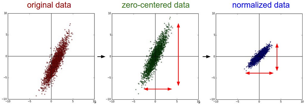
Data Preprocessing
Data: $[X]_{NxD}$, where $N$ is the number of data, $D$ is the dimensionality
Mean Subtraction
Center the data around origin along every dimension
X -= np.mean(X, axis=0)
X -= np.mean(X) # images
Normalization
normalize so that data is approximately the same scale
Divide Zero-centered data with Standard Deviation
	X /= np.std(X, axis=0)
  	X /= np.std(X)
Min-Max
- Normalize so that Min is $-1$ and Max is $+1$
- Apply only when different input features have different scale but equally important to the learning algorithm
- For images, not necessary as images are in range of (0,255)
- PCA and Whitening
Preprocessing statistics (mean and std) must be computed based on the training data and then to be applied on the validation and test data
Weights Initialization
- All Zeros Initialization - Pitfall
- Final value of every weight in trained network is not known
- With proper data normalization, we can assume that half of weights will be +ve and half will be -ve.
- Setting all initial weights to zero is a mistake, since then every neuron will compute same output and gradients will also be same and so same updates.
Small Random Numbers
We still want weights close to zero
If neurons are all random and unique, they will compute distinct updates and integrate themselves as diverse parts of the full network
# randn gives random numbers from zero mean and unit standard deviation gaussian
W = 0.01 * np.random.randn(D, H)
Little impact if numbers drawn from uniform distribution
Warning
- Small weights may create problem due to fact that their gradients will also be smaller and may diminish for deep networks
Calibrating the variances with 1/sqrt(n)
- Variance in the outputs from randomly initialized neuron grows with the number of inputs.
- We can normalize variance of each neuron’s output by scaling its weight vector by sqrt of its fan-in (inputs)
- $w = \frac{np.random.randn(n)}{sqrt(n)}$
- This ensures that all neurons initially have approximately the same output distribution and empirically improves the rate of convergence.
- Let $s = \sum\limits_{i}^{n} w_i.x_i$, now
- $Var(s) = \sigma^2(s) = \sum\limits_{i}^{n} \sigma^2(w_i.x_i)$
- $\sigma^2(s) = \sum\limits_{i}^{n} [\sigma^2(w_i).\sigma^2(x_i) + {\mathop{\mathbb{E}}(w_i)}^2.\sigma^2(x_i)] + \sigma^2(w_i).{\mathop{\mathbb{E}}(x_i)}^2 $
- Since, we have zero mean inputs and weights, $\mathop{\mathbb{E}}(w_i)=0,~ \mathop{\mathbb{E}}(x_i)=0$
- This is not general, as ReLU units will have positive mean
- $\sigma^2(s) = \sum\limits_{i}^{n} \sigma^2(w_i).\sigma^2(x_i) $
- $\sigma^2(s) = n .\sigma^2(w).\sigma^2(x) $
- If we want $s$ to have the same variance as $x$, then we make sure that variance of every $w$ is $1/n$
- Thus, we initialize $w = np.random.randn(n) / sqrt(n)$
- He et al. reached the conclusion that the variance of neurons in the network should be $2/n$
- This gives initialization $w = np.random.randn(n) . sqrt(\frac{2.0}{n})$
- This is current recommendation with ReLU Neurons
Sparse Initialization
- Set all weight matrices to zero but connect every neuron to fixed number of neurons below it (randomly connected with weights sampled from a small gaussian).
Initialization Biases
- Since asymmetry breaking is provided by weights, biases can be initialized to zero.
- For ReLU, some prefer to initalize bias with 0.01 to ensure that all ReLU units obtain and propogate gradients. No evidence if it benefits
- Insert a BatchNorm Layer after fully connected or convolutional layers and before non-linearity.
- This explicitly force activations throughout the network and to take on a unit Gaussian distribution at the beginnning of the training.
- Network with BN are more robust to bad initialization
Regularization
Helps to prevent overfitting to control capacity of Neural Network.
L2 Regularization
- Penalize the squared magnitude of all parameters in the objective
- We add $\frac{1}{2}\lambda w^2~\forall~w$, where $\lambda$ is the regularization strength. 1/2 is added to make gradient $\lambda w$ instaed of $2\lambda w$.
- Thus, it heavily penalizes peak weight vectors and prefer diffuse weight vectors. It encourages the network to use all of its weights rather than using some a lot.
- During gradient descent parameter update, L2 means that every weight is decayed linearly $ w = w - \lambda w$ towards zero
L1 Regularization
- In L1, we add $\lambda w~\forall~w$ in the obejctive function
- Elastic net regularization combines L1 and L2
- $\lambda_1w+\lambda_2w^2$
- Neurons with L1 will end up using only a sparse subset of important inputs and become invariant to noisy inputs
- If we are not concerned with explicit feature selection then L2 gives better performance
Max norm Constraints
$ \overrightarrow{w} _2 < c$, where $c$ may be of order 3 or 4 - It enforces an absolute upper bound on the magnitude of the weight vector for every neuron and use projected gradient descent to enforce the constraint.
- Network cannot explode even with high learning rates
Dropout complements L1, L2, and maxnorm
Keep a neuron active during training with some probability $p$ and setting to zero otherwise. $p$ is a hyper parameter
It can be interpreted as sampling a network from full Neural Network, and only updating the parameters of the sampled network.
- The exponential number of possible sampled networks are not independent because they share the parameters
During testing, there is no dropout, with interpretation of evaluating an averaged prediction across the exponentially-sized ensemble of all sub-networks.
p = 0.5
def train_step(X):
  h1 = np.dot(W1, X) + b1
  h1 = np.maximum(0, h1)
  u1 = np.random.rand(*h1.shape) < p # dropout mask
  h1 = h1 * u1

  h2 = np.dot(W2, h1) + b2
  h2 = np.maximum(0, h2)
  u2 = np.random.randn(*h2.shape) < p # dropout mask
  h2 = h2 * u2

  out = np.dot(W3, h2) + b3
  # Backward pass, compute gradient
  # Perform Parameter update

def predict(X):
  h1 = np.dot(W1, X) + b1
  h1 = np.maximum(0, h1)
  h1 = h1 * p # Scale the activation
  h2 = np.dot(W2, h1) + b2
  h2 = np.maximum(0, h2)
  h2 = h2 * p # Scale the activation
  out = np.dot(W3, h2) + b3
Dropout can also be applied on the input layer
In the predict function, we are not dropping but applying scaling by p.
- Scaling is important since at test time all neurons see their inputs, and we want the outputs of neurons at test time to be identical to their expected output at training time.
- If p =0.5, neurons must halve the output at the test time to have the same output as during training
Since test-time performance is critical, it is preferable to use inverted dropout, which performs scaling during train time and leaving the forward pass at test time untouched
p = 0.5
def train_step(X):
  h1 = np.dot(W1, X) + b1
  h1 = np.maximum(0, h1)
  u1 = np.random.rand(*h1.shape) < p # dropout mask
  u1 = u1 / p
  h1 = h1 * u1

  h2 = np.dot(W2, h1) + b2
  h2 = np.maximum(0, h2)
  u2 = np.random.randn(*h2.shape) < p # dropout mask
  u2 = u2 / p
  h2 = h2 * u2

  out = np.dot(W3, h2) + b3
  # Backward pass, compute gradient
  # Perform Parameter update

def predict(X):
  h1 = np.dot(W1, X) + b1
  h1 = np.maximum(0, h1)

  h2 = np.dot(W2, h1) + b2
  h2 = np.maximum(0, h2)

  out = np.dot(W3, h2) + b3
Theme of noise in forward pass
- Dropout falls into category of methods that introduce stochastic behavior in the forward pass of the network
- During testing, noise is marginalized over analytically (by multiplying p) or numerically (sampling and several forward passes and then averaging)
- Another direction is the DropConnect, where random set of weights is instead set to zero during forward pass.
- CNN take adavntage of DropConnect with Stochastic Pooling, Fractional Pooling, and Data Augumentation
Bias Regularization
- It is not common to regularize the bias parameters as they don’t interact with data through multiplicative interactions and so son’t have the interpretation of controlling the influence of data on the objective function
- However, since bias parameters are few in comparison to weights, so regularizing bias rarely leads to worst performance. Classifier can afford to use biases if it needs them to obtain better loss
Per-Layer Regularization
- It is not common to regularize different layers to different amounts (except output layer)
- Few publications on this
In Practice
- Use a single global L2 regularization strength that is cross-validated
- Also common to combine this with dropout applied after all layers
- p=0.5 is default can can be tuned on the validation data
Loss Functions
- Regularization penalizes the model complexity
- Loss function mesaures compatibility between prediction and ground truth
- $L = \frac{1}{N}\sum\limits_{i} L_i$
- Let $f=f(x_i;W)$ be the activations of the output layer in a Neural Network
- Classification
- Single correct label out of a fixed set
- SVM Loss, $L_i = \sum\limits_{j\ne y_i} max(0, f_j+1-f_{y_i})$
- Squared Hinge Loss, $L_i = \sum\limits_{j\ne y_i} max(0, f_j+1-f_{y_i})^2$
- Cross Entropy Loss used by softmax classifier, $L_i=-log\big(\frac{e^{f_{y_i}}}{\sum\limits_{j} e^{f_j}} \big)$
- Problem: Large number of classes
- Softmax probs becomes expensive when labels are large
- For certain applications, approximate versions are popular
- Attribute Classification
- When correct class $y_i$ is not a single answer but a binary vector where the attributes are not exclusive
- Sensibile approach is to build binary classifier for every single atttribute independently
- $L_i = \sum\limits_{j} max(0, 1-y_{ij}f_j)$


