Fast Gradient Sign Attack
Published:
This post covers MNIST implementation of ICLR 2015 paper “Explaining and Harnessing Adversarial Examples”
Source: PyTorch
Import Libraries
import torch
import torch.nn as nn
import torch.nn.functional as F
import torch.optim as optim

from torchvision import datasets, transforms

import numpy as np
import matplotlib.pyplot as plt

%matplotlib inline

device = 'cuda' if torch.cuda.is_available() else 'cpu'
print(device)
Pretrained Model
pretrained_model = 'model/lenet_mnist_model.pth'
epsilons = [0, 0.05, .1, .15, .2, .25, .3]
LeNet Model
class Net(nn.Module):
    def __init__(self):
        super(Net, self).__init__()
        self.conv1 = nn.Conv2d(1, 10, kernel_size=5)
        self.conv2 = nn.Conv2d(10, 20, kernel_size=5)
        self.conv2_drop = nn.Dropout2d()
        self.fc1 = nn.Linear(320, 50)
        self.fc2 = nn.Linear(50, 10)

    def forward(self, x):
        x = F.relu(F.max_pool2d(self.conv1(x), 2))
        x = F.relu(F.max_pool2d(self.conv2_drop(self.conv2(x)), 2))
        x = x.view(-1, 320)
        x = F.relu(self.fc1(x))
        x = F.dropout(x, training=self.training)
        x = self.fc2(x)
        return F.log_softmax(x, dim=1)
MNIST Test Dataset
tfs = [transforms.ToTensor()]
transform = transforms.Compose(tfs)

ds_test = datasets.MNIST(root='data', download=True, train=False, transform=transform)

loader_test = torch.utils.data.DataLoader(ds_test, batch_size=1, shuffle=True)
Load Pretrained Model
# Initialize the network
model = Net().to(device)

model.load_state_dict(torch.load(pretrained_model, map_location=device))

model.eval()
FSGM Attack
- Rather than working to minimize the loss by adjusting the weights based on the backpropagated gradients, the attack adjusts the input data to maximize the loss based on the same backpropagated gradients.
- In other words, the attack uses the gradient of the loss w.r.t the input data, then adjusts the input data to maximize the loss.
def fgsm_attack(image, epsilon, data_grad):
    sign_data_grad = data_grad.sign()

    perturbed_image = image + epsilon * sign_data_grad

    perturbed_image = torch.clamp(perturbed_image, 0, 1)

    return perturbed_image
Test Module
def test(model, loader_test, epsilon):
    correct = 0
    adv_examples = []

    for data, target in loader_test:

        data, target = data.to(device), target.to(device)

      	data.requires_grad = True # For attack

        output = model(data)
        pred_init = output.max(1, keepdim=True)[1]

        if pred_init.item() != target.item():
            continue # No need to attack if model pred is not correct

        loss = F.nll_loss(output, target)
        loss.backward()
        model.zero_grad()

        data_grad = data.grad.data

        data = fgsm_attack(data, epsilon, data_grad) # perturbed image

        output = model(data)
        pred_final = output.max(1, keepdim=True)[1]

        if pred_final.item() != target.item(): # Attack successful
            if len(adv_examples) < 5:
                adv_ex = data.squeeze().detach().cpu().numpy()
                adv_examples.append((pred_init.item(), pred_final.item(), adv_ex))
        else:
            correct += 1 # Attack Unsuccessful
            if len(adv_examples) < 5 and epsilon == 0: # save only when eps is 0 when attack not successful
                adv_ex = data.squeeze().detach().cpu().numpy()
                adv_examples.append((pred_init.item(), pred_final.item(), adv_ex))
    acc = correct*1.0 / len(loader_test)
    print('Eps: {} \t Accuracy = {}/{}={:.3f}'.format(epsilon, correct, len(loader_test), acc))
    return acc, adv_examples
Run Test
accuracies = []
examples = []

for eps in epsilons:
    acc, ex = test(model, loader_test, eps)

    accuracies.append(acc)
    examples.append(ex)
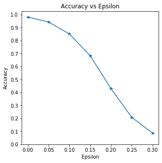
Eps: 0 Accuracy = 9810/10000=0.981 Eps: 0.05 Accuracy = 9426/10000=0.943 Eps: 0.1 Accuracy = 8510/10000=0.851 Eps: 0.15 Accuracy = 6826/10000=0.683 Eps: 0.2 Accuracy = 4301/10000=0.430 Eps: 0.25 Accuracy = 2082/10000=0.208 Eps: 0.3 Accuracy = 869/10000=0.087
print(epsilons)
print(accuracies)
[0, 0.05, 0.1, 0.15, 0.2, 0.25, 0.3] [0.981, 0.9426, 0.851, 0.6826, 0.4301, 0.2082, 0.0869]
Visualization
plt.figure(figsize=(5,5))

plt.plot(epsilons, accuracies, '*-')

plt.yticks(np.arange(0, 1.1, step=0.1))
plt.xticks(np.arange(0, .35, step=0.05))
plt.title("Accuracy vs Epsilon")
plt.xlabel("Epsilon")
plt.ylabel("Accuracy");
plt.figure(figsize=(8,10))

cnt = 0
for i in range(len(epsilons)):
    for j in range(len(examples[i])):
        cnt += 1
        plt.subplot(len(epsilons), len(examples[i]), cnt)
        orig, adv, ex = examples[i][j]

        plt.imshow(ex, cmap='gray')

        plt.xticks([], [])
        plt.yticks([], [])
        plt.title("{} -> {}".format(orig, adv))

        if j == 0:
            plt.ylabel("Eps: {}".format(epsilons[i]), fontsize=14)

plt.tight_layout()
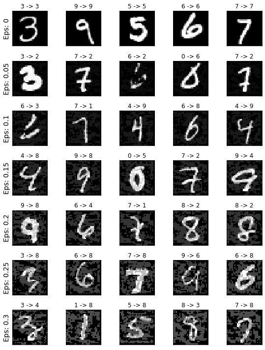
- All correct for Eps 0 row