This post explains ANOVA.

F-table

Comparing Samples

• Which of the products have significantly different prices
  • Product A and Product B
  • Product A and Product C
  • Product B and Product C
  • No significant difference
• How many t-tests would we need to compare for 4 samples A, B, C, D
  • 6 (AB, AC, AD, BC, BD, AD)
  • $\binom{n}{2} = \frac{n!}{2!(n-2)!}$

$tStatistic = \frac{\bar{X_1}-\bar{X_2}}{\sqrt{\frac{S_1^2}{n_1}+\frac{S_2^2}{n_2}}}$

Compare three or more samples = $\frac{distance/variability~between~means}{error}$

• To compare three or more samples

  • Find the average squared deviation of each sample mean from the total mean
    • like std
  • Total Mean or Grand Mean $\bar{X_G}$
  • Samples sizes equal
    • $\bar{X_G} = \text{Mean of sample means} = \frac{\bar{X_1} + \bar{X_2}+…+\bar{X_n}}{n}$
    • or
    • $\bar{X_G} = \text{Mean of sample means} = \frac{X_1 + X_2+…+X_N}{N}$
  • If not equal
    • $\bar{X_G} = \text{Mean of sample means} = \frac{X_1 + X_2+…+X_N}{N}$

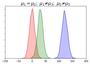
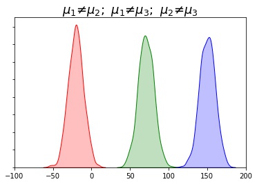
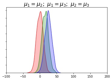
• Between-group Variability

  • Conclusions from the deviation of each sample mean from the mean of means
    • Smaller the distance between sample means, the less likely population means will differ significantly
    • Greater the distance between sample means, the more likely population means will differ significantly

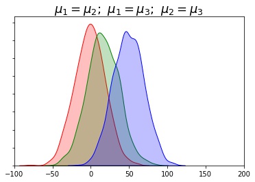
• Within-group Variability

• In which situation are the means significantly different

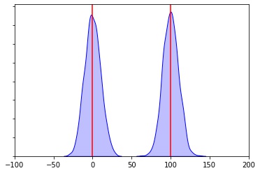
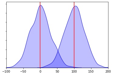
  • Less Variablity	More Variablity

  • Greater the variability of each individual sample, the less likely population means will differ significantly

  • The smaller the variability of each individual sample, the more likely population means will differ significantly

Aalysis of Variance (ANOVA)

• One Test to compare $n$ means
• One-way ANOVA
  • One Independent Variable
• Two-way ANOVA
  • Two Independent Variable

One-way ANOVA

• $H_0: \mu_1 = \mu_2 = \mu_3$
• $H_A:$ At least one pair of samples is significantly different
  • If we get small statistic => Within-group > Between-group => means are not significantly different from each other => Fail to reject the Null
  • If we get large statistic => Within-group < Between-group => means are significantly different from each other => Reject Null
• Higher Within-group variability is in favour of Null Hypothesis
• Higher Between-group variability is in favor of Alternate Hypothesis
• Ratio
  • Numerator = Between-group
  • Denominator = Within-group
• $F = \frac{between-group~variability}{within-group~variability}$

Example

ANOVA

• Between-group variability $ = \frac{n\Sigma(\bar{X_k}-\bar{X_G})^2}{k-1} $

• Within-group Variability $ = \frac{\Sigma(X_i-\bar{X_k})^2}{N-k} $, where $N$ is the total number of values from all samples and $k$ the number of Samples
• $F = \frac{\frac{n\Sigma(\bar{X_k}-\bar{X_G})^2}{k-1}}{\frac{\Sigma(X_i-\bar{X_k})^2}{N-k}} = \frac{\frac{SS_{betweeb}}{df_{between}}}{\frac{SS_{within}}{df_{within}}} = \frac{MS_{between}}{MS_{within}}$
  • SS - Sum of Squared
  • MS - Mean Squared
• $df_{total} = df_{between} + df_{within} = N - 1$
• $SS_{total} = \Sigma(x_i-\bar{X_G})^2 = SS_{between} + SS_{within}$
• $F$-statistic is never negative
  • not symmatrical
  • positively skewed
  • Peakes at 1 since if no difference between population means then between-group and within group will be same
  • Always No Direction $\ne$
  • Critical region on right side only

Example

• Is there significant differences in prices of items from three brands based on data of prices of some random shirts

  • [15, 12, 14, 11]
  • [39, 45, 48, 60]
  • [65, 45, 32, 38]

• Hypothesis

  • $H_0: \mu_1 = \mu_2 = \mu_3$
  • $H_A:$ At least one pair of samples is significantly different

• brand1 = [15, 12, 14, 11]
  brand2 = [39, 45, 48, 60]
  brand3 = [65, 45, 32, 38]
    
  n = 4 # Sample Size
  k = 3 # No of samples
    
  xbar1 = np.mean(brand1) # 13.00
  xbar2 = np.mean(brand2) # 48.00
  xbar3 = np.mean(brand3) # 45.00
    
  xbarG = (xbar1 + xbar2 + xbar3)/3 # 35.33
    
  print(f'xbar1={xbar1:.2f}, xbar2={xbar2:.2f}, xbar3={xbar3:.2f}, xbarG={xbarG:.2f}')
  # xbar1=13.00, xbar2=48.00, xbar3=45.00, xbarG=35.33
    
  xbars = [xbar1, xbar2, xbar3]
    
  SSbetween = []
  for xbar in xbars:
      ss = (xbar-xbarG)**2
      SSbetween.append(ss)
  SSbetween = n * sum(SSbetween) # 3010.67
  #SSbetween = n * sum([(xbar-xbarG)**2 for xbar in xbars])
  print(f'SSbetween = {SSbetween:.2f}') # 3010.67
    
    
  SSwithin1 = np.sum([(val - xbar1)**2 for val in brand1])
  SSwithin2 = np.sum([(val - xbar2)**2 for val in brand2])
  SSwithin3 = np.sum([(val - xbar3)**2 for val in brand3])
  SSwithin = SSwithin1 + SSwithin2 + SSwithin3
  print(f'SSwithin = {SSwithin:.2f}')
  # SSwithin = 862.00
    
  dfbetween = k - 1 # 2
  dfwithin = n * k - k # 9
  print(f'dfbetween = {dfbetween} dfwithin = {dfwithin}')
  # dfbetween = 2 dfwithin = 9
    
  MSbetween = SSbetween / dfbetween
  MSwithin = SSwithin / dfwithin
    
  print(f'MSbetween = {MSbetween:.2f} MSwithin = {MSwithin:.2f}')
  # MSbetween = 1505.33 MSwithin = 95.78
    
  Fstatistic = MSbetween / MSwithin
  print(f'Fstatistic = {Fstatistic:.2f}')
  # Fstatistic = 15.72
    
  # http://www.socr.ucla.edu/Applets.dir/F_Table.html
  # col = 2 row = 9 alpha = 0.05
  Fcritical = 4.2565
    
  from scipy import stats
  alpha = 0.05
  Fcritical = stats.f.ppf(1-alpha, dfn=dfbetween, dfd=dfwithin)
  print(f'Fcritical = {Fcritical:.4f}')
  # Fcritical = 4.2565
    
  Fstatistic > Fcritical
  print('Reject Null in favor of Alternate')
  

  Fstatistic, pvalue = stats.f_oneway(brand1, brand2, brand3)
  print(f'Fstatistic = {Fstatistic:.2f} pvalue={pvalue:.4f}')
  # Fstatistic = 15.72 pvalue=0.0012

Two-way ANOVA

• The only difference between one-way and two-way ANOVA is the number of independent variables. A one-way ANOVA has one independent variable, while a two-way ANOVA has two.
• used to determine whether or not there is a statistically significant difference between the means of three or more independent groups that have been split on two factors.
• The purpose of a two-way ANOVA is to determine how two factors impact a response variable, and to determine whether or not there is an interaction between the two factors on the response variable.
• For example, suppose a botanist wants to explore how sunlight exposure and watering frequency affect plant growth. She plants 30 seeds and lets them grow for two months under different conditions for sunlight exposure and watering frequency. After two months, she records the height of each plant.
• Response variable
  • plant growth
• Factors
  • sunlight exposure, watering frequency
• Questions
  • Does sunlight exposure affect plant growth?
  • Does watering frequency affect plant growth?
  • Is there an interaction effect between sunlight exposure and watering frequency? (e.g. the effect that sunlight exposure has on the plants is dependent on watering frequency)
• Two-Way ANOVA Assumptions

• 1. Normality – The response variable is approximately normally distributed for each group.

  2. Equal Variances – The variances for each group should be roughly equal.

  3. Independence – The observations in each group are independent of each other and the observations within groups were obtained by a random sample.

Example

import numpy as np
import pandas as pd

#create data
df = pd.DataFrame({'water': np.repeat(['daily', 'weekly'], 15),
                   'sun': np.tile(np.repeat(['low', 'med', 'high'], 5), 2),
                   'height': [6, 6, 6, 5, 6, 5, 5, 6, 4, 5,
                              6, 6, 7, 8, 7, 3, 4, 4, 4, 5,
                              4, 4, 4, 4, 4, 5, 6, 6, 7, 8]})

print(df.shape)
df.sample(10)

# !pip3 install statsmodels
import statsmodels.api as sm
from statsmodels.formula.api import ols

#perform two-way ANOVA
model = ols('height ~ C(water) + C(sun) + C(water):C(sun)', data=df).fit()
sm.stats.anova_lm(model, typ=2)

• Interpret the results.
  • We can see the following p-values for each of the factors in the table:
    • water: p-value = .000527
    • sun: p-value = .0000002
    • water*sun: p-value = .120667
  • Since the p-values for water and sun are both less than .05, this means that both factors have a statistically significant effect on plant height.
  • since the p-value for the interaction effect (.120667) is not less than .05, this tells us that there is no significant interaction effect between sunlight exposure and watering frequency.